Mlsys Memo
- Mlsys Memo
- DNN Architecture
- Modern DL, computational graph, autodiff, frameworks
- Dataflow Graph Representation
- Autodiff
- Graph Optimization
- Arithmetic Intensity
- Parallelization
- Optimize Arithmetic Intensity
- Operator Acceleration
- Matrix Multiplication
- GPU Matmul and Operator Compilation
- Triton, graph optimization and compilation
- Memory
- Parallelization
- Data Parallelism
- Intra-operator Parallelism
- Few More Optimizations for parallelism
- Auto-parallelization
- Hao’s ultimate guide
- Parallelism to LLM training
DNN Architecture
key considerations of mapping from algorithmic requirements to computer system design:
- Memory access patterns: How data moves through the memory hierarchy
- Computation characteristics: The nature and organization of arithmetic operations
- Data movement: Requirements for on-chip and off-chip data transfer
- Resource utilization: How computational and memory resources are allocated
metrics for system impplications:
- memory requirements
- computation needs
- data movement
MLP: Dense Pattern Processing
MLPs process each input element with equal importance, making them versatile but computationally intensive.
Situations: any input feature could potentially influence any output—there are no inherent constraints on these relationships, demanding an architectural pattern capable of learning arbitrary relationships across all input features.
Dense pattern processing:
- addresses this fundamental need by enabling:
- allows unrestricted feature interactions where each output can depend on any combination of inputs
- facilitates learned feature importance, allowing the system to determine which connections matter rather than having them prescribed.
- provides adaptive representation, enabling the network to reshape its internal representations based on the data.
CNN: Spatial Pattern Processing
Spatial pattern processing addresses scenarios where the relationship between data points depends on their relative positions or proximity.
CNNs use a local connection pattern where each output connects only to a small, spatially contiguous region of the input.
RNN: Sequential Pattern Processing
Transformer: Dynamic Pattern Processing
Modern DL, computational graph, autodiff, frameworks
DL Computation
DL Workloads
most important models:
- Convolutional neural networks
- Recurrent neural networks
- Transformers
- Mixture-of-Experts
most important optimization algorithms:
- SDG
- Adam
- …
Most important components in CNN
- Conv layer
- Conv1d, Conv2d, Conv3d
- MatMul
- Softmax
- element-wise operations
- ReLU, add, sub
- Pooling
Most important components in RNN
- Matrix multiplication. Required for updating the internal states and for forward propagation.
- Element-wise nonlinear activations. ReLU, tanh, and sigmoid functions are frequently used in RNNS.
Most important components in Transformer
- Transformers = Attention + MLP + something else
- Attention:
- Matmul
- Softmax
- Normalization
- MLP:
- Matmul
- Something else:
- Layernorm, GeLU, etc.
Most important components in Mixture-of-Experts
The only novel component in MoE is something called a router. Because the model is replicated across multiple experts, you need to embed a router to determine which expert will process each input.
The router is constituted by the following operations:
- Matmul
- Softmax
Matmul (plus Softmax) are all you need. MLSys ≈ Matmul Systems
High-level pictures:
- We have data xi for i = 1 to n, represented as tensors in memory.
- We have our model, which consists of mathematical primitives (primarily matmul). The model represents the computation through these primitives.
- We have compute, which ensures the programs run on clusters of different types of hardware.
Dataflow Graph Representation
OLAP: Online Analytical Processing vs OLTP: Online Transaction Processing
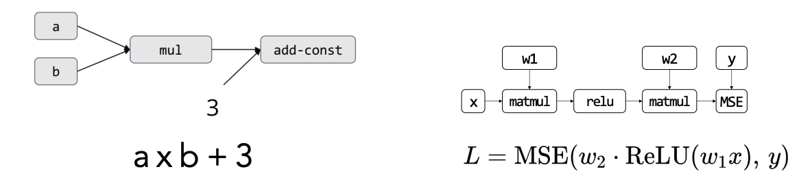
Computational Dataflow Graph
represents the flow of computation in a ML pipeline
- Node: represents the computation (operator)
- Edge: represents the data dependency (data flowing direction)
- Node: also represents the output tensor of the operator
- Node: also represents an input constant tensor (if it is not a compute operator)
Case study: TensorFlow
-
In TensorFlow, the forward computation, loss function, autodiff, and SGD update rule are first declared in code. The real execution is triggered as the last step. Behind the scenes, TF is building a static CDG as it declares each component, which the execution then follows strictly.
-
The benefits of building a dataflow graph using this method are that abstracting a pipeline or series of computations as a CDG can allow us to capitalize on opportunities for parallelism and optimization, since different branches of the graph can be run in parallel.
-
However, there are also some drawbacks. It is difficult to model dynamic computations with static dataflow graphs. In static CDGs, the graph is fully defined before execution (as TF does), representing a rigid structure that strictly follows the predefined computations and data flow.
Case study: Pytorch
- Pytorch implements a solution to the above problem. Instead of pre-defining the CDG before execution, it creates the graph as the forward operations are executed. It then uses the resultant graph during backpropagation. However, this flexibility comes at the cost of increased computational overhead because the graph is recreated every forward pass.
Symbolic vs. Imperative
Symbolic Programming
requires declaring and defining all symbols before executing any tasks. pros:
- easier to optimize, offering features like distributed processing, parallelization, and batching.
- Symbolic frameworks are typically the most efficient way to write a program, often achieving up to 10 times greater efficiency. cons:
- counterintuitive, making debugging more challenging
- need to be defined first before proceeding with the actual task making it harder to code and debug, as well as being less flexible
Imperative Programming
a programming paradigm where the code explicitly defines the steps required to solve a problem
code is defined in a way that justifies each action needed to solve the problem
pros:
- easier to debug and understand
- very flexible cons:
- less efficient than symbolic programming
- harder to optimize
Why is Python Imperative while TensorFlow is Symbolic?
- TensorFlow relies on a domain-specific language (DSL) built on top of Python
- PyTorch’s DSL is more Pythonic than TensorFlow’s
Just-in-time (JIT) Compilation
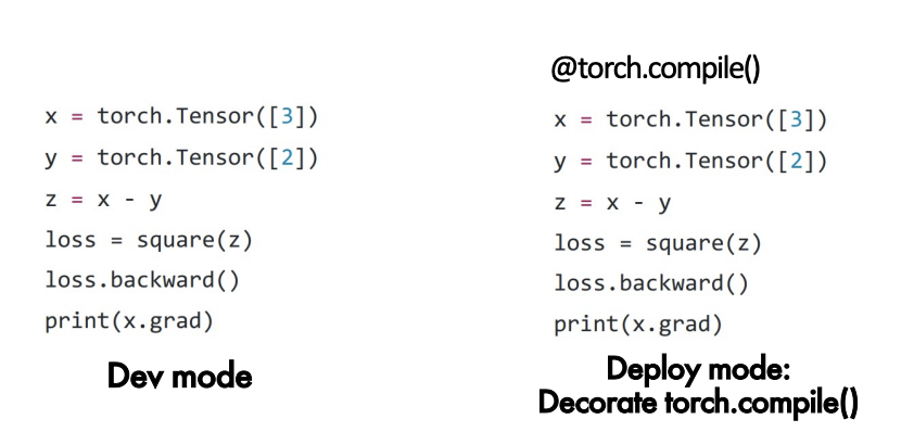
JIT compilation combines the flexibility of define-and-run during development with the efficiency of definethen-run during deployment.
Define-and-run
Provides:
- a flexible environment to Experiment with models and algorithms.
- Easily debug using print statements and interactive tools.
Define-then-run
Once the model is finalized, we prioritize performance:
- The code should run efficiently without interactive modifications.
- The decorator @torch.compile() converts the dynamic PyTorch code into a static, optimized graph.
- Static graph resembles TensorFlow’s execution model.
JIT Compilation in PyTorch
- using
torch.compile()to convert the dynamic PyTorch code into a static, optimized graph for deployment. - Once the code is locked down, add torch.compile() as a decorator to optimize the model.
- The optimized graph improves performance but can no longer be altered with tools like print statements.
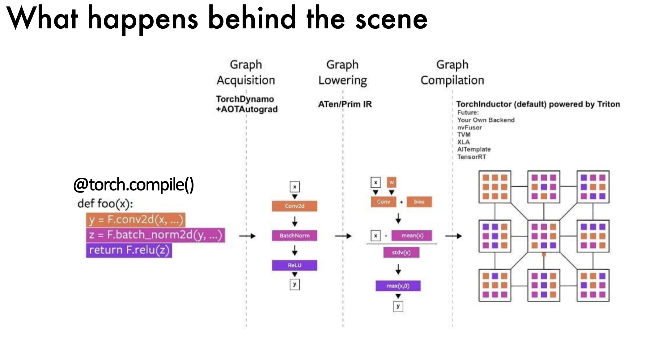
- Graph Acquisition: The first step is to acquire the graph, using TorchDynamo and AOTAutograd to transform the dynamic code into a computation graph.
- Graph Lowering: The second step is to lower the graph, using ATen/Prim IR to convert the graph into a lower-level representation.
- Graph Compilation: The third step is to compile the graph, using TritonInductor to generate optimized code for the target hardware.
JIT Compilation Problem
JIT compilation can only be used on a static execution graph
- struggles with very dynamic programs, i.e. those with frequent if/else branching, might cause graph structure changes
- Static graphs prevent dynamic debugging and reduce flexibility.
JIT compilation is best suited for models that can be locked down into a static graph. Highly dynamic behavior may reduce its effectiveness.
Static Models vs. Dynamic Models
Static Dataflow Graphs
dataflow graph remains unchanged regardless of the input data
- requires that both the input and output data have fixed shapes.
- Define once, optimized once, execute many times
- Execution: Once defined, all following computation will follow the defined computation
Dynamic Dataflow Graphs
dataflow graph changes based on the input data
- Difficulty in expressing complex flow-control logic
- Complexity of the computation graph implementation
- Difficulty in debugging
- just-in-time (JIT) compilation is nearly impossible for programs relying on dynamic graphs
example: in Semantic Parsing Trees for NLP, the structure of the parsing tree differs for each input sentence
Methods to handle dynamic models
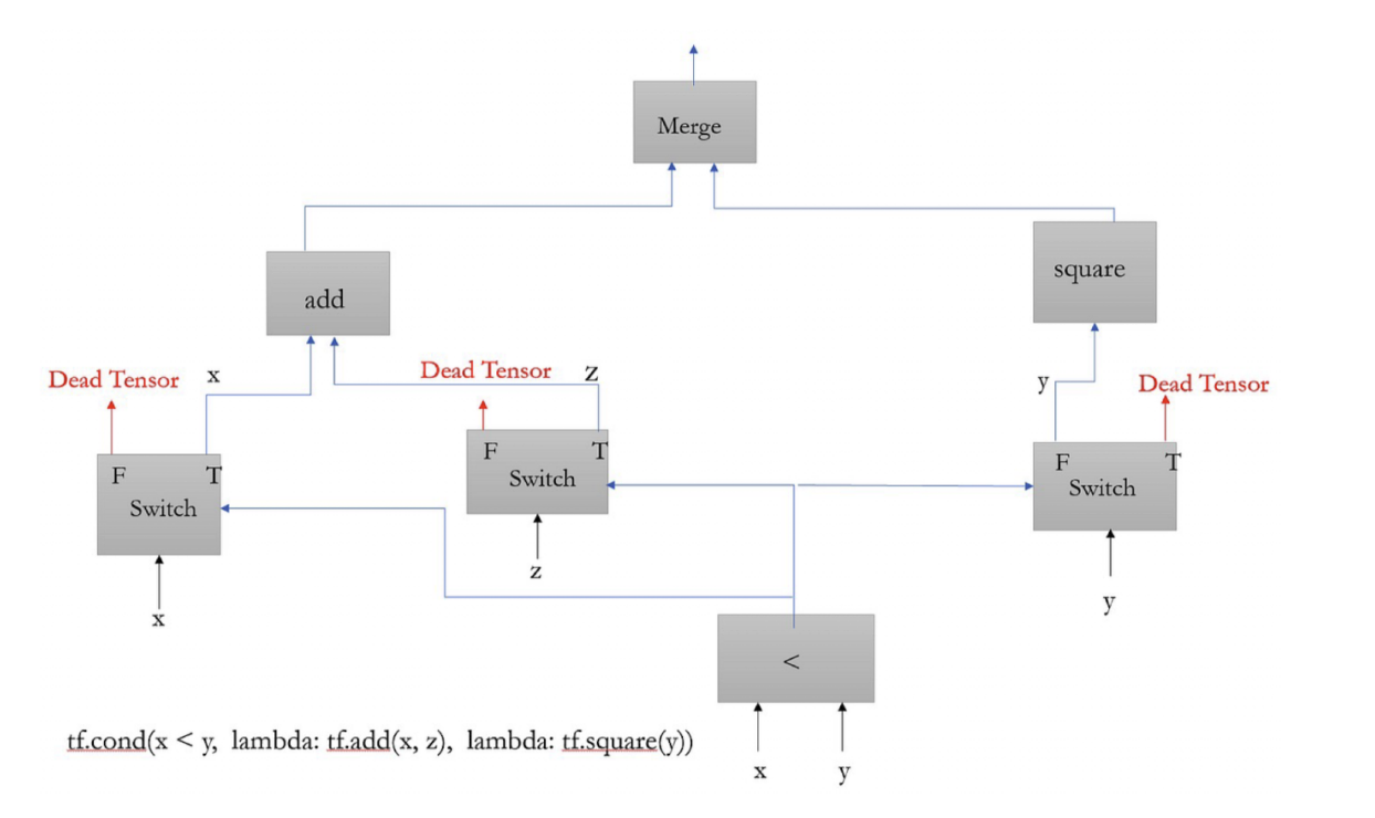
- Control Flow Operations: a fundamental concept in programming languages
- primitive: Switch and Merge

- The Switch operation determines whether to pass the input data or output a dead tensor based on a boolean predicate.
- Conversely, the Merge operation takes two inputs and outputs the one that is not a dead tensor.
- possible problems:
- Deriving gradients for control flow operations (ie. switch, fork) can be challenging, although it is feasible.
- Adding control flow increases the complexity of the dataflow graph.
- Piecewise Compilation:
- case1: How can we apply static JIT compilation to a graph that accepts input shapes of
[x, c1, c2]where c1 and c2 are constants and x is a variable?- Compile for All Possible Input Dimensions:
- pre-compile multiple graphs, each corresponding to a specific value of x
- select the graph that matches the input dimensions at runtime.
- Bucketing with Power of 2:
- compile graphs for input shapes where x aligns with powers of 2 (e.g., x = 1, 2, 4, 8, …).
- At runtime, the input dimensions are mapped to the closest ceiling power of 2 bucket.
- This reduces the number of pre-compiled graphs compared to the first approach, offering a balance between flexibility and resource utilization.
- Compile for All Possible Input Dimensions:
- case2: How can we apply static JIT compilation to a graph that is static first, dynamic next, and then static?
- introducing guards at the boundaries of the static and dynamic sections.
- Insert guards at the end of the first static section and the beginning of the second static section.
- Compile the static sections into binary files.
- Execute the first static binary, pass its result into the dynamic section (which runs in pure Python), and feed the dynamic output into the second static binary for further processing.
- introducing guards at the boundaries of the static and dynamic sections.
- case1: How can we apply static JIT compilation to a graph that accepts input shapes of
Autodiff
- autodiff uses symbolic differentiation
- using PD: sum, product, and chain rules
Forward Mode Autodiff
- start from the input nodes and derive the gradient all the way to the output nodes.
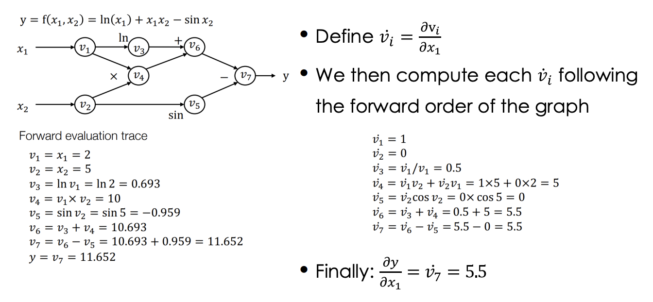
- in ML, usually the input dimension n is large, while the output dimension k is 1 or small
- forward mode autodiff is not as effective for ML
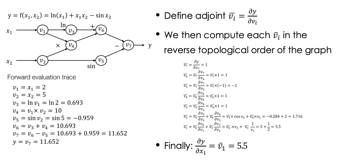
Reverse Mode Autodiff
-
- Start from the output nodes
- Derive gradient all the way back to the input nodes
- Discussion: Pros and Cons of FM Autodiff?
- For 𝑓: 𝑅𝑛 → 𝑅𝑘, we need 𝑘 backward passes to get the grad w.r.t. each input
- in ML: 𝑘 = 1 and 𝑛 is very large
Backpropagation vs Reverse AD
The summary of Backward AD:
- Rather than working directly with concrete values (numerical computations), the backward graph symbolically represents the operations involved, enabling the automatic computation of derivatives.
- Once the backward graph is constructed, it can be reused for different sets of input values. This allows efficient computation during training processes in machine learning models, especially neural networks.
- Popular machine learning libraries like TensorFlow and PyTorch utilize backward automatic differentiation to compute gradients efficiently. This functionality enables optimization algorithms like gradient descent to update model parameters.
Reverse mode AD:
- creates a bigger graph, which captures both the forward computations and the reverse gradient propagation in a symbolic form. This graph structure is commonly used by modern frameworks such as TensorFlow and PyTorch because it allows for efficient computation of derivatives with respect to many inputs simultaneously, a necessity for large-scale machine learning models.
- In contrast, backpropagation (used in frameworks like Caffe and CUDA-convnet) focuses solely on computing the gradient for a specific function or layer. While effective for basic gradient computation, backpropagation lacks the flexibility and reusability provided by reverse mode AD, especially for complex scenarios.
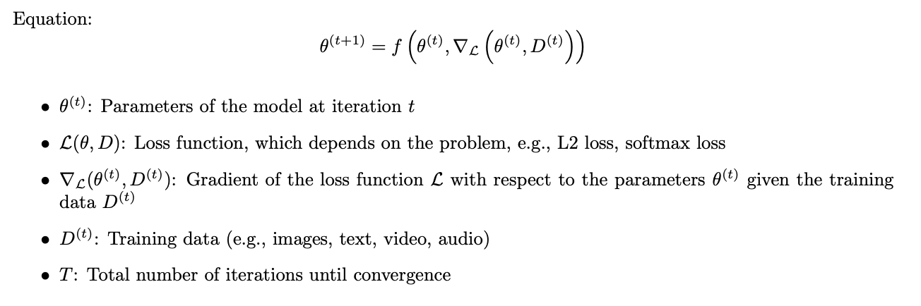
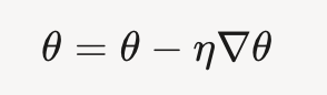
weight updates
- weight updates are performed after computing the gradients
- using rule of gradient descent:
- 𝑤 = 𝑤 - 𝜂 * ∂𝐿/∂𝑤
- where 𝑤 is the weight, 𝜂 is the learning rate, and ∂𝐿/∂𝑤 is the gradient of the loss function with respect to the weight.
Graph Optimization
Intuition: The graph written by the user might be inefficient, the system will take the graph defined by the user, try to analyze it and optimize it so that the graph will be more efficient.
- Rewrite the original graph G to G’
- G’ runs faster than G
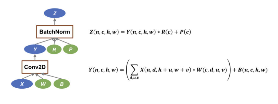
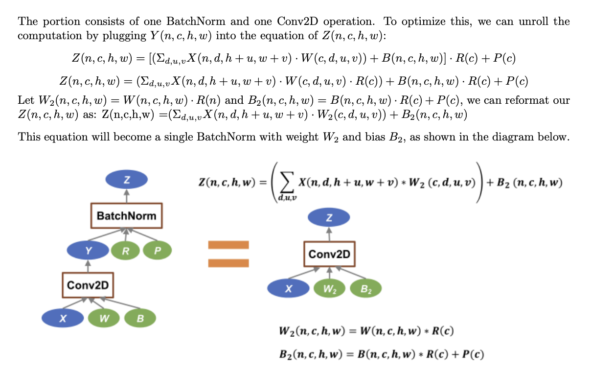
- BatchNorm + Conv2D
- Fusing MatMul and Add
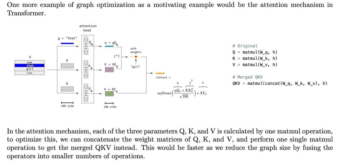
- Transformer QKV concatenate
Arithmetic Intensity
Arithmetic Intensity: AI = #ops / #bytes
- the ratio of total operations over total data movements
- The higher the arithmetic intensity, the better / more efficient the algorithm is.
- example:
  void add(int n, float* A, float* B, float* C){
    for (int i = 0; i < n; i++)
    C[i] = A[i] + B[i]
  }
Algorithm: Read A[i] Read B[i] Add A[i] + B[i] Stores C[i]- 1 compute and 3 read/writes −> 1/3
- example
float *A, *B, *C, *D, *E, *tmp1, *tmp2; //Algorithm 1: add(n, A, B, tmp1); mul(n, tmp1, C, tmp2); add(n, tmp2, D, E); //Algorithm 2: void fused(int n, float* A, float* B, float* C, float* D, float* E){ for (int i=0; i<n; i++){ E[i] = D[i] + (A[i] + B[i]) * C[i]; } } fused(n, A, B, C, D, E)- Arithmetic Intensity for Algorithm 1: 3 compute and 9 read/writes −> 1/3
- Arithmetic Intensity for Algorithm 2: 3 compute and 5 read/writes −> 3/5
Parallelization
- partition the computational graph on the device cluster
- locality vs parallelism
Optimize Arithmetic Intensity
Key Focus
- Vectorization: uses hardware instructions to process multiple data points simultaneously, reducing execution time.
- Data Layout Optimization: The way data is stored in memory (row-major vs. column-major) affects access speed. Aligning data with the memory hierarchy improves cache use and accelerates read/write operations.
- Parallelization: Splitting tasks across multiple cores or threads speeds up processing. GPUs excel here, using thousands of cores to handle large computations quickly.
Vectorization
 // unvectorized code
  float A[256], B[256], C[256];
  for (int i = 0; i < 256; ++i) {
    C[i] = A[i] + B[i];
  }

  // vectorized code
  for (int i = 0; i < 64; ++i) {
    float4 a = load_float4(A + i*4);
    float4 b = load_float4(B + i*4);
    float4 c = add_float4(a, b);
    store_float4(C + i*4, c);
  }
looping 256 times to perform the operation -> only need to loop 64 times
Data Layout
- Row-Major vs Column-Major
- strides format:
- example:
  A[i0][i1][i2]... = A_internal[
    stride offset
    + i0 * A.strides[0]
    + i1 * A.strides[1]
    + i2 * A.strides[2]
    + ...
    + in-1 * A.strides[n-1]
  ]
// Example of a 2D A[i, j] = A.data[offset + i * A.strides[0] + j * A.strides[1]] - offset and strides
- Offset: indicates the offset of the tensor relative to the underlying base storage
- Strides: is an array of the same shape as the total number of dimensions of the tensor (i.e., len(strides) = A.shape). Strides[i] indicate how many elements need to be skipped in memory in order to move “one-unit” in the ith dimension of the tensor.
- If the underlying storage of an array A is row-major,
strides = [A.shape[1], 1] - If the underlying storage of an array A is col-major,
strides = [1, A.shape[0]]
- Benefits of using the Strides format: Zero-Copy
- Strides separate the underlying storage and the view of the tensor.
- can perform various tensor operations by just changing how the data is accessed (via stride values) rather than moving or duplicating the data in a new memory location
- like: slicing, transpose, broadcasting
- Permute/Transpose: Strides format helps achieve permute operations by modifying the strides array values.
- Slice: This operation is achieved by manipulating both the offset values and the strides array values.
- Broadcast: The only thing that changes to achieve broadcasting is the strides array.
- example:
Operator Acceleration
Using strides to accelerate operators
Slicing
changing:
- offset
- shape
- strides
example: slicing a 4 x 5 matrix into a 3 x 2 matrix
- original matrix:
A = [[a00, a01, a02, a03, a04], [a10, a11, a12, a13, a14], [a20, a21, a22, a23, a24], [a30, a31, a32, a33, a34]]- Identify the sub-matrix: suppose slicing the sub matrix starts at row 1, column 2, and has shape 3 × 2, like
B = [[a12, a13], [a22, a23], [a32, a33]] - Compute the new metadata
- offset = 1 * 5 + 2 = 7:
- 1 * 5: the first row has 5 elements, so we skip the first row
- 2: the second column has 2 elements, so we skip the first two columns - shape = (3, 2) - strides = (5, 1):
- Row-major strides were [5, 1].
- The sub-matrix is still laid out row by row, so strides = [5, 1] in this view.
- Identify the sub-matrix: suppose slicing the sub matrix starts at row 1, column 2, and has shape 3 × 2, like
Transpose
- 2d example:
[m,n] -> [n,m] - higher dimensional example:
[m,n,k] -> [k,m,n]
two ways of transposing:
- Logical (Stride-Based) Transpose (Zero-Copy):
- 2D example:
- Original strides might be
stride_row, stride_col = [n, 1]for an[m, n]array. - swap the strides to
stride_row, stride_col = [1, m]for transposing the array. - no cost of copying data, but less cache-friendly
- Physical Transpose (Copy):
- This gives better memory locality for many operations on the transposed data but requires time and memory to perform the copy.
Most deep-learning or numerical frameworks (NumPy, PyTorch, TensorFlow, etc.) support both ways.
.T (NumPy) or .transpose(...) (PyTorch/TensorFlow) often defaults to returning a view (stride-based transpose) if it can. But if a contiguous buffer is needed for performance, they might materialize (copy) the transposed tensor.
Broadcasting
example: adding a and b with a.shape = [4, 3] and b.shape = [1, 3]
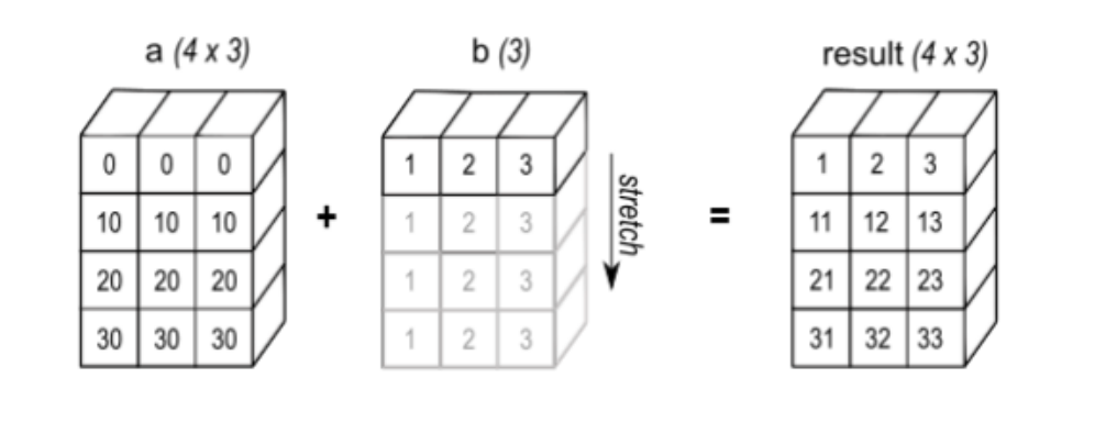
- Rudimentary way: Copy four times. It is slow and consumes a lot of memory
- How we really implement it: Change b.stride from
[1]to[0, 1]; and b.shape from[1, 3]to[4, 3]- by doing so, with
A.strides[0] = 0, we haveA[i, j] = A.data[offset + j × A.strides[1]] for any i
- by doing so, with
- In practice, Pytorch does this for us automatically behind the scenes when we input
a + bora @ b
Pitfall of stride: discontinuity
Using stride can easily violate that requirement. For example, when we create a new tensor by slicing an existing tensor, the storage of this new tensor in the memory is essentially discontinuous as we skip some elements stored in between.
This is why we have contiguous method in Pytorch.
summary for operator acceleration:
- Vectorization
- Data Layout Optimization
- CPU Parallelization
Matrix Multiplication
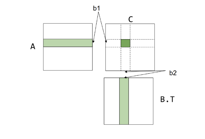
Cache-aware Tiled Matrix Multiplication
- Cache-Aware Tiling: This strategy focuses on efficiently transferring data between DRAM and the L1 cache.
- code example
-
dram float A[n / b1 ][ b1 ][ n ]; dram float B[n / b2 ][ b2 ][ n ]; dram float C[n / b1 ][ n/ b2 ][ b1 ][ b2 ]; for (int i = 0; i < n/ b1 ; ++ i) { l1cache float a [0: b1 , 0: n] = A[i ]; for (int j = 0; j < n/ b2 ; ++ j) { l1cache float b [0: b2 , 0: n] = B[j ]; C[i][j] = dot (a , b.T); // Register - aware tiling can be applied here for further optimization } } - cost analysis:
- Reads Between DRAM and L1 Cache for Matrix A:
(n/b1)*n*b1 = n^2
- Reads Between DRAM and L1 Cache for Matrix B:
(n/b1)*(n/b2)*b2*n = n^3/b1
- Total Cost:
Total Cost = n^2 + n^3/b1
- L1 cache size constraint
b1*n + b2*n <= L1_cache_size
- Reads Between DRAM and L1 Cache for Matrix A:
Register-aware Tiling
- Register-Aware Tiling: This strategy deals with moving data from the L1 cache to the processor registers.
- code example
-
dram float A[n/ v1 ][ n / v3 ][ v1 ][ v3 ]; dram float B[n/ v2 ][ n / v3 ][ v2 ][ v3 ]; dram float C[n/ v1 ][ n / v2 ][ v1 ][ v2 ]; for (int i = 0; i < n/ v1 ; ++ i) { for (int j = 0; j < n/ v2 ; ++ j) { register float c[ v1 ][ v2 ] = 0; for (int k = 0; k < n/ v3 ; ++ k) { register float a [0: v1 , 0: v3 ] = A[i ][ k ]; register float b [0: v2 , 0: v3 ] = B[j ][ k ]; c += dot (a , b .T); } C[i][j] = c; } } - cost analysis:
- the total read operation for A is:
- `(n/v1)(n/v2)(n/v3)v1v3 = n^3/v2
- The total read operations for B is:
(n/v2)*(n/v3)*(n/v1)*v2*v3 = n^3/v1
- For C:
n^2(since C is written once for each i, j pair)
- The total number of registers needed:
v1*v3 + v2*v3 + v1*v2 <= register_size
- the total read operation for A is:
- Comparison with Cache-aware Tiling:
- In the untiled implementation of matrix multiplication, space usage in the L1 cache is minimal, as data is loaded directly from DRAM into the registers for computation without intermediate buffering. However, this simplicity comes at a significant performance cost, as the process requires n^3 read operations for both matrices A and B, leading to substantial redundant memory accesses. In contrast, cache-aware tiling leverages the L1 cache to store tiles of A, B, and C, enabling extensive data reuse and reducing the number of redundant memory accesses. Specifically, the total cost of cache-aware tiling is n^2 + n^3/b1 , which is significantly lower than the untiled version for reasonable tile sizes (b1 and b2). While cache-aware tiling requires additional L1 cache space proportional to the tile sizes (b1 · n + b2 · n), this trade-off results in significantly improved I/O efficiency and computational performance by reducing data transfer overhead between DRAM and the L1 cache.
Combine Together
- In the untiled implementation of matrix multiplication, space usage in the L1 cache is minimal, as data is loaded directly from DRAM into the registers for computation without intermediate buffering. However, this simplicity comes at a significant performance cost, as the process requires n^3 read operations for both matrices A and B, leading to substantial redundant memory accesses. In contrast, cache-aware tiling leverages the L1 cache to store tiles of A, B, and C, enabling extensive data reuse and reducing the number of redundant memory accesses. Specifically, the total cost of cache-aware tiling is n^2 + n^3/b1 , which is significantly lower than the untiled version for reasonable tile sizes (b1 and b2). While cache-aware tiling requires additional L1 cache space proportional to the tile sizes (b1 · n + b2 · n), this trade-off results in significantly improved I/O efficiency and computational performance by reducing data transfer overhead between DRAM and the L1 cache.
-
dram float A[n / b1 ][ b1 / v1 ][ n ][ v1 ]; dram float B[n / b2 ][ b2 / v2 ][ n ][ v2 ]; for (int i = 0; i < n/ b1 ; ++ i) { l1cache float a[ b1 / v1 ][ n ][ v1 ] = A[ i ]; for (int j = 0; j < n/ b2 ; ++ j) { l1cache float b[ b2 / v2 ][ n ][ v2 ] = B [j ]; for (int x = 0; x < b1 / v1 ; ++ x) { for (int y = 0; y < b2 / v2 ; ++ y) { register float c [ v1 ][ v2 ] = {0}; for (int k = 0; k < n; ++ k) { register float ar [0: v1 ] = a [x ][ k ][:]; register float br [0: v2 ] = b [y ][ k ][:]; C += dot (ar , br .T) ; } } } } } - Cache Tiling (Outer Loops): Parameters b1 and b2 are used to divide the computation into tiles that fit into L1 cache, reducing the need to repeatedly fetch data from DRAM.
- Register Tiling (Inner Loops): Parameters v1 and v2 further divide the tiles into smaller chunks that fit into registers, minimizing L1 cache to register traffic.
- DRAM → L1 Cache
cost = (n/b1)*(b1/v1)*n*b1 = n^2cost = (n/b1)*(n/b2)*(b2/v2)*n*v2 = n^2/b1
- Cost: l1 -> register:
(n/b1) * (n / b2) * (b1 / v1) * (b2/ v2) * n * v1 = n^3 / v2n^3 / v1
Key Questions for Optimization
- Parameter Selection
- v1, v2 are register tiling parameters and should fit within the available registers.
- b1, b2 are cache tiling parameters and must fit within L1 or L2 cache.
- Concurrent Reads:
- Non-blocking caches and hardware/software prefetching can enable overlapping data movement at different levels.
- Pipelining memory transfers and computation ensures efficient resource utilization.
Why Tiling Works: Reuse Loading
- reusing data across multiple computations, thereby reducing redundant memory accesses
- example:
C[i][j] = sum(A[i][k] * B[j][k], axis=k);- In matrix multiplication, accessing
A[i][k]is independent of the j-dimension. By tiling along the j-dimension:- We can reuse
A[i][k]for multiple computations ofC[i][j]. - This reduces the number of times A needs to be fetched from memory.
- We can reuse
- Reduced Memory Bandwidth, Increased Cache Efficiency (less misses), Improved Performance
Hardware Accelerator
CPU Parallelization
- SIMD, see memo for parallelism
GPU Parallelization
GPU and CUDA
basic terminology
- GPU
- Threads: lowest-level workers in GPU computing and execute instructions concurrently within a warp.
- warps: A group of 32 threads (usually on Nvidia GPUs) that execute instructions simultaneously in a Single Instruction, Multiple Thread (SIMT) model. Warps are the standard scheduling unit in a streaming multiprocessor.
- SIMT: Single Instruction, Multiple Threads, a parallel computing model used in GPUs where multiple threads execute the same instruction simultaneously, threads-level parallelism
- Blocks: A collection of threads that share memory. Each block is assigned to a single streaming multiprocessor (SM/SMP). The SM schedules and executes the threads in warps (usually 32 threads per warp).
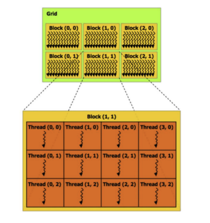
- Grid: A collection of blocks that execute the same kernel. The grid defines the total structure of threads involved in the computation.
- Kernel: A function written in CUDA (or any other GPU programming framework) that is executed by many threads on the GPU in parallel. Each thread executes the kernel with a unique thread ID so that they can operate on different portions of data.
-
Steaming Multiprocessors: Each SM can handle a set number of blocks and threads. Therefore, adding more SMs will result in higher computational throughput (throughput refers to the amount of computational work a system can complete in a given period of time; the faster the better).
- relations: Kernel -> Grid -> Block -> warp -> Thread
- kernel: a function that runs on the GPU, entry point for GPU execution
- Grid: a collection of blocks, which can be distributed across multiple SMs. Kernel execution is defined by the grid.
- Block: a collection of threads, assigned to a single SM. Thread within a block can communicate with each other through shared memory.
- warp: a collection of threads, the smallest unit of execution in a GPU. Threads within a warp execute the same instruction with different data.
- Thread: the smallest unit of execution in a GPU, each thread has its own registers and local memory.
- CUDA
- Host Code: Host code refers to the portion of the program that runs on the computer’s CPU. It is responsible for:
- Managing the overall program flow
- Allocating and deallocating memory on both the host (CPU) and device (GPU)
- Transferring data between the host and device
- Launching kernel functions to be executed on the GPU
- Synchronizing CPU and GPU operations
- Host code is written in standard C or C++ and is compiled using a regular C/C++ compiler.
- Device Code: Device code, on the other hand, is the part of the program that runs on the GPU. It consists of:
- Kernel functions: Special functions that are executed in parallel on the GPU
- Device functions: Helper functions that can only be called from within kernel functions or other device functions
- Host Code: Host code refers to the portion of the program that runs on the computer’s CPU. It is responsible for:
CUDA Code Example
  // This part of code runs on CPU
  // Host code: serial execution on CPU
  // Data dimensions
  const int Nx = 12;
  const int Ny = 6;

  dim3 threadsPerBlock(4, 3, 1); // 12 threads per block

  // set blocks needed
  dim3 numBlocks(Ns/threadsPerBlock.x, Ny/threadsPerBlock.y, 1); // (3, 2, 1) = 6

  // the following call triggers execution of 72 CUDA threads
  // “launch a grid of CUDA thread blocks” Call returns when all threads have terminated
  matrixAddDoubleB<<<numBlocks, threadsPerBlock>>>(A, B, C);
- params:
- GridDim - Dimensions of the grid.
- blockIdx - The block index within the grid.
- blockDim - The dimensions of a block.
- threadIdx - The thread index within a block.
- CUDA kernel for the above code:
__device__ float doubleValue(float x) { return 2 * x; } // kernel definition // __global__ indicates that this function runs on the GPU //Each thread indexes its data using blockIdx, blockDim, threadIdx and execute the compute //Device code: SIMD parallel execution GPUs //kernel functions must have a void return type because they’re executed by multiple threads in parallel. __global__ void matrixAddDoubleB(float A[Ny][Nx], float B[Ny][Nx], float C[Ny][Nx]) { int i = blockIdx.x * blockDim.x + threadIdx.x; int j = blockIdx.y * blockDim.y + threadIdx.y; C[j][i] = A[j][i] + doubleValue(B[j][i]); } - Synchronization: The kernel execution is asynchronous
- CPU program continues executing without halting while the device code runs on the GPU
- the device code mustn’t have any return values—causes erroneous behavior.
- To get results from the GPU,
CUDA.synchronizeis used (simplest way, cause CPU to wait until all threads are done) cudaMemcpyis used to copy data from the GPU to the CPU
- Data Map:
- It is the user’s responsibility to ensure that the job is correctly partitioned and the memory is handled correctly.
- The blockDim, shapes, etc., should be statically declared.
- This is the reason why compilers like torch.compile require static shapes.
- important to check the boundry conditions of the data
- SIMD Constraints: handle control flow
- requires all ALUs/cores to process at the same pace.
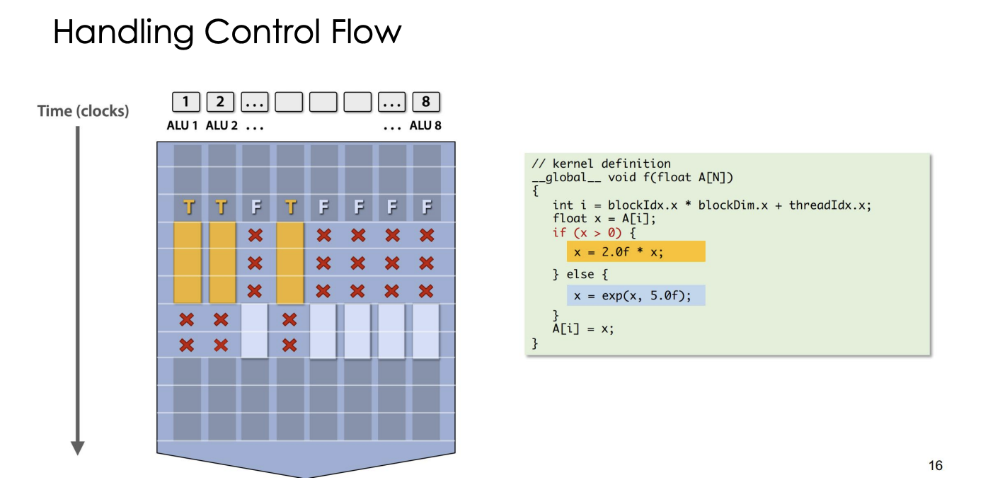
- threads in same warp have to execute the same instruction
- Control Flow Divergence: when encountering a branch, threads in the same warp diverge, executing different instructions serially
- This sequence introduces idle cycles—often called “bubbles”—and can diminish efficiency.
- Coherent vs. Divergent
- Coherent execution:
- Same instructions apply to all data
- Divergence Execution:
- On the contrary of coherent
- Should be minimized in CUDA programs
- Coherent execution:
CUDA Memory Model
- HBM: High Bandwidth Memory
- a specialized memory technology that delivers significantly higher speed and bandwidth compared to traditional CPU memory
- GPU memory uses a memory pool model optimized for parallelism, allowing multiple threads to access memory concurrently
- pinned memory:
- a dedicated portion of host memory optimized for high-speed data transfers between the CPU and GPU
- locked and non-pageable, for more efficient GPU access
CUDA Memory Hierarchy
- Global memory (HBM):
- resides in the GPU’s device memory
- accessible to all threads
- largest storage capacity but comes with higher latency and slower access times
- for data that is infrequently accessed or shared across the entire grid
- Shared memory:
- a high-speed memory allocated per thread block
- shared among all threads within the block
- significantly faster access than global memory but is limited in size
- for intermediate computations and data shared between threads in the same block
- Private memory:
- threads’ own local private memory
- limited to thread-local operations
- the fastest access speeds
CUDA Memory Access Example
- original code:
for i in range(len(input) - 2): output[i] = (input[i] + input[i + 1] + input[i + 2])/3.0 - host code:
int N = 1024*1024; cudaMalloc(&devInput, sizeof(float)*(N+2)); // To account for edge conditions cudaMalloc(&devOutput, sizeof(float)*N); convolve<<<N/THREADS_PER_BLK, THREADS_PER_BLK>>>(N, devInput, devOutput); - device code
#define THREADS_PER_BLK = 128 __global__ void convolve(int N, float* input, float* output) { int index = blockIdx.x *blockDim.x + threadIdx.x; float result = 0.0f; //thread-local variable result = input[index] + input[index + 1] + input[index + 2]; output[index] = result /3.f; } - problem:
- each element is read thrice
- the number of blocks assigned is much more than what a typical GPU has,
oversubscribed
- Optimized version
#define THREADS_PER_BLK = 128 __global__ void convolve(int N, float* input, float* output) { int index = blockIdx.x *blockDim.x + threadIdx.x; __shared__ float support[THREADS_PER_BLK+2]; support[threadIdx.x] = input[index]; if(threadIdx.x < 2){ support[THREADS_PER_BLK + threadIdx.x] = input[index + THREADS_PER_BLK]; } __syncthreads(); float result = 0.0f; //thread-local variable for(int i=0; i<3; i++) result += support[threadIdx.x + i]; output[index] = result /3.f; }__shared__indicates that the variable is shared among threads in the same block__syncthreads()is used to synchronize all threads in the block, ensuring that all threads have completed their operations on the shared memory before proceeding- By using shared memory, we can decrease number of memory operations:
- In this case, we use 128 threads to calculate 128 outputs which only cost us 128 + 2 = 130 memory operations. However, without using shared memory, we need 128 × 3 = 384 memory operations to generate the same 128 results.
CUDA Compilation
A compiled CUDA device binary includes:
- Program text (instructions)
- Information about required resources:
- For example, a program might require - 128 threads per block, 8 types of local data per thread and 130 floats (520 bytes) of shared space per thread block.
Resource Management Issue:
- different GPUs have different SMs or number of threads.
- the amount of resources available differs between GPUs.
Solution: Dynamic Scheduling
- A more feasible solution is that CUDA schedules the thread blocks to many cores (SMs), using a dynamic scheduling policy that respects the resource requirements. It assumes that the thread blocks are not dependent on each other, and can be executed in any order.
The scheduler works as follows: blocks are assigned according to the available resources, and the remaining ones are queued. Whenever a scheduled block is finished, the next block in the queue is scheduled in the finished block’s place. The scheduler is dynamic because it can assign blocks to cores depending on the current situation, rather than working with a fixed, predetermined schedule.
GPU Matmul and Operator Compilation
CUDA Thought Process
- identify the work that can be parallelized.
- partition the task and identify the subset of data that is associated with each partition and bind pair to a CUDA thread
- Implement the logic in the CUDA kernel and the GPU will launch the code into multiple threads under the hood.
make sure:
- Oversubscription: create enough tasks to keep all execution units on a machine busy
- Mitigate straggler: Balance workload (because GPU cores does not know control flow), We need to balance the workload across the thread as equal as possible such that each thread has same amount of workload. We need to avoid If-else conditional statements at all costs.
- Minimize “communication”: reduce I/O across memory hierarchies
Case: Matmul Optimization
GPU Matmul v1
C = A x B
simplified version of code:
- kernel code
__global__ void mm(float A[N][N], float B[N][N], float C[N][N]) { int x = blockIdx.x * blockDim.x + threadIdx.x; int y = blockIdx.y * blockDim.y + threadIdx.y; float result = 0.0f; for (int k = 0; k < N; ++k) { result += A[x][k] * B[k][y]; } C[x][y] = result; } - host code
  int N = 1024;
  dim3 threadsPerBlock(32, 32, 1);
  dim3 numBlocks(N/32, N/32, 1);
  mm<<<numBlocks, threadsPerBlock>>>(A, B, C);
threadsPerBlock(32, 32, 1)specifies a block of 32*32=1024 threads.numBlocks(N/32, N/32, 1)indicates how many blocks cover the full NN matrix. For N=1024, this is (32,32) blocks. The total number of threads is (3232)(3232)=1024*1024=1,048,576
Memory Access and Performance Analysis
- single thread needs to fetch the entire x-th row of A (size N) and the entire y-th column of B (also size N) to compute the dot product. This equates to N + N = 2N floating-point reads per thread.
- There are N^2 threads (one for each C-element). Total read operations can be around N^2 ×2N = 2N^3 which is very large for bigger N
- Storing A, B, and C each requires N^2 floats in global memory.
GPU Matmul v1.5
to have each thread compute an entire V x V submatrix instead of only 1 entry
- Essentially this means that we divide the original N x N resulting matrix into a grid of N/V x N/V blocks.
-
Thus, each block is of size V x V. Within each of these blocks, we then compute each of these V^2 entries.
- code:
__global__ void mm(float A[N][N], float B[N][N], float C[N][N]) { int xbase = blockIdx.x * blockDim.x + threadIdx.x; int ybase = blockIdx.y * blockDim.y + threadIdx.y; float c[V][V] = {0}; float a[N], b[N]; for (int x = 0; x < V; ++x) { a[:] = A[xbase * V + x, :]; for (int y = 0; y < V; ++y) { b[:] = B[:, ybase * V + y]; for (int k = 0; k < N; ++k) { c[x][y] += a[k] * b[k]; } } } C[xbase * V: xbase * V + V, ybase * V: ybase * V + V] = c[:]; } - Thus, for the overall matrix of size N x N, this method requires (N/V)^2 = N^2/V^2 threads and each thread requires NV + NV^2 memory reads.
- Thus, the total global memory access requires is (N^2/V^2)(NV + NV^2) = N^3/V + N^3 memory reads.
- to compute the values of the whole V x V block, the local memory required must increase to V^2 + 2N floats per thread
GPU Matmul v2
- code:
__global__ void mm(float A[N][N], float B[N][N], float C[N][N]) { int xbase = blockIdx.x * blockDim.x + threadIdx.x; int ybase = blockIdx.y * blockDim.y + threadIdx.y; float c[V][V] = {0}; float a[V], b[V]; for (int k = 0; k < N; ++k) { a[:] = A[xbase * V: xbase * V + V, k]; b[:] = B[k, ybase * V: ybase * V + V]; for (int y = 0; y < V; ++y) { for (int x = 0; x < V; ++x) { c[x][y] += a[x] * b[y]; } } } C[xbase * V: xbase * V + V, ybase * V: ybase * V + V] = c[:]; } 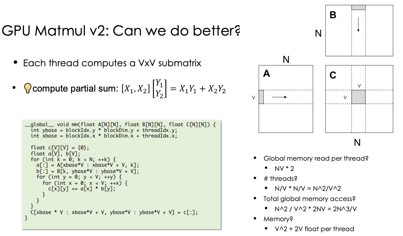
- Global memory reads per thread: NV × 2
- Number of threads: N^2/V^2
- Total global memory access: (N^2/V^2) × 2NV =2N^3/V
- Memory requirement per thread: V^2 + 2V floats, covering the registers used for computation.
GPU Matmul v3: SRAM Tiling
- code:
__global__ void mm(float A[N][N], float B[N][N], float C[N][N]) { __shared__ float sA[S][L], sB[S][L]; float c[V][V] = {0}; float a[V], b[V]; int yblock = blockIdx.y; int xblock = blockIdx.x; for (int ko = 0; ko < N; ko += S) { __syncthreads(); // needs to be implemented by thread cooperative fetching sA[:, :] = A[ko : ko + S, yblock * L : yblock * L + L]; sB[:, :] = B[ko : ko + S, xblock * L : xblock * L + L]; __syncthreads(); for (int ki = 0; ki < S; ++ ki) { a[:] = sA[ki, threadIdx.y * V : threadIdx.y * V + V]; b[:] = sA[ki, threadIdx.x * V : threadIdx.x * V + V]; for (int y = 0; y < V; ++y) { for (int x = 0; x < V; ++x) { c[y][x] += a[y] * b[x]; } } } } int ybase = blockIdx.y * blockDim.y + threadIdx.y; int xbase = blockIdx.x * blockDim.x + threadIdx.x; C[ybase * V : ybase*V + V, xbase*V : xbase*V + V] = c[:]; }- Line 2 in the code uses the
__shared__keyword to declare sA and sB in shared memory. - sA and sB will hold the S × L regions which are loaded in each iteration.
- In this code sB is declared as an S × L array even though the region is L × S
co-operative fetching: However the way sA and sB are loaded here is not correct. In this implementation every thread will load the entire S × L block. In reality we need to partition the loading between threads so that each thread only loads one part.- The second
__syncthreadsis needed so that all threads have finished loading their part (remember the actual implementation is through co-operative fetching). -
The first
__syncthreadsis needed in case a thread which finishes the remainder of the loop faster than others and starts loading the regions for the next iteration. - We load one N × L region each from A and B so the total global memory access for one block is 2NL.
- There are N^2/L^2 blocks and so the total global memory access is 2NL × (N^2/L^2) = 2N^3/L
- Each thread loads two S × V regions in each iteration of the loop. But ultimately the thread needs to load the entire region of size N × V in both A and B in order to calculate Cthread (of size V × V ). So the memory access for a thread is 2VN.
- There are N2 V 2 threads and so the total shared memory access is 2VN × N^2/V^2 = 2N^3/V
- Line 2 in the code uses the
Other Optimizations
- Cooperative Fetching: all threads in a block work together to load data into shared memory, reducing redundant memory accesses and improving performance.
- Continuous read: Reading off of offsets is slow
- avoid bank conflicts: Bank conflicts occur when multiple threads access the same memory bank simultaneously, leading to serialization and performance degradation. To avoid bank conflicts, ensure that threads access different banks or use padding to distribute accesses evenly across banks.
- pipeline threads: some threads do reading and some threads do computation
- Tensor Core
- Lower precision
Core Problem for CUDA
- kernel tuning:
- How should we decide L (block sub-matrix size) and V (matrix computed by thread)?
- depends on the number of threads, number of registers, and the amount of SRAM available on the system
- kernel tuning: The process of determining the optimal hyperparameters for a kernel
- when PyTorch or Tensorflow is loaded, it automatically determines (profiles your system for) the optimal hyperparameters based on your system.
usually use a machine learning based compilers that take the compiler, code, and devices and automatically determine the optimized implementation for operations.
Machine Learning Compilers
primary goal: automatically generate optimal configurations and kernel code from high-level code (e.g., TensorFlow, PyTorch, Python) for target hardware.
Traditional Compilers vs. ML Compilers
- Traditional Compilers:
- Input: Human-written code focusing on general-purpose programming languages
- Process: transforming it into machinereadable instructions optimized for specific hardware
- Output: Machine instructions executed by hardware
- ML Compiler:
- Input: User-defined ML models in frameworks, represented as dataflow graphs
- Process: Compilers automatically transform dataflow graphs into an optimized version and generates efficient kernel code for various operators used within the graph. Additionally, they use existing compilers, such as CUDA, to produce hardware-specific machine code
- Output: Optimized machine code for efficient execution of ML workloads
Possible Problems
- Programming-level issues: Using arbitrary, imperative user code to generate compile-able code can be very challenging due to the difficulties in transforming highly dynamic user-code into static dataflow graphs
- Graph-level issues: Optimizing and transforming dataflow graphs automatically to make it faster
- Operator-level issues: Generating efficient kernel code for individual operators on diverse hardware
Notable ML Compilers
- XLA
- TVM
- torch.compile, was introduced as part of PyTorch 2.0
- Modular
Operator Compilation
Problem Definition
- Possibilities: How to represent the search space (low-level program variants) and all possibilities?
- Searching: How to find the closest-to-optimal value in the search space? (enumerate many possibilities)
- Acceleration: How to reduce the search space for efficiency?
- Generalizability: How to generalize the search on different hardwares?
case study: AutoTVM
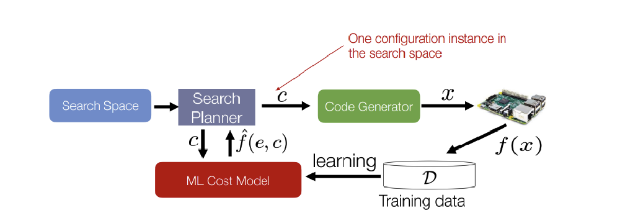
- Search Space: pre-defined possible combinations of configurations for each operator
- Search Planner: Enumerate through the space.
- Code Generator: Compile kernel codes based on user’s code and hardware specifications.
- Cost Model: Apply the codes on target hardware and model its performance, e.g. using neural networks to generalize and predict the performance, taking loop parameters as the input of the function and performance as the output of the function.
Template-based Search Space: experts to write a template, i.e. writing the skeleton codes and leaving the looping factors as parameters for compiler optimization.
Searching Strategies:
- Early Pruning the search space: pruning the bad performance candidates in the early stages of searching
- Cost Modeling: using historical data to predict the performance of loops on target hardware
Triton, graph optimization and compilation
Triton
High-level DSL for CUDA
Device-specific DSL vs Compiler:
- DSL:
- advantage: users have high flexibility when developing kernels. They can use whatever data-structures and low-level techniques that can squeeze the last bits of performance.
- disadvantage: the development process requires deep expertise, and it’s really hard and time-consuming to write correct and fast kernels.
- Compiler:
- advantage: users can write kernels quickly and prototype ideas at high iteration speed
- disadvantage: compilers cannot represent certain types of ideas involving in-operator control flow and custom data structures
- Performance Cliffs: compiler frameworks depends highly on templates and pattern matching, which can lead to performance cliffs when the compiler cannot find the right template for the user’s code.
- In-Operator Control Flow: if operator has dynamic control flow or runtime if-else statements, it is hard for the compiler to optimize the code.
- Custom Data Structures: compilers usually assume that the data structures are structured tensor, if complex data structures are used, it is hard for the compiler to optimize the code.
- Triton:
- On development difficulty, Triton is Python based and simpler than Cuda.
- On expressing ability, Triton is less expressive than Cuda, but more expressive than graph compilers.
Triton Programming Model
The programming model of Triton is based on several ideas:
- Triton is embedded in Python, and kernels are defined with triton.jit decorator.
- Users construct tensors of pointers in SRAM, and modify them elementwise with torch-like primitives.
- The tensors must have power-of-two number of elements along each dimension, otherwise Triton will do the padding.
  import triton.language as tl
  Import triton
  @triton.jit
  def _add(z_ptr, x_ptr, y_ptr, N):
    # same as torch.arrange
    offsets = tl.arange(0, 1024)
    # create 1024 pointers to X, Y, Z
    x_ptrs = x_ptr + offsets
    y_ptrs = y_ptr + offsets
    z_ptrs = z_ptr + offsets
    # load 1024 elements of X, Y, Z
    x = tl.load(x_ptrs)
    y = tl.load(y_ptrs)
    # do computations
    z = x + y
    # write-back 1024 elements of X, Y, Z
    tl.store(z_ptrs, z)
  N = 1024
  x = torch.randn(N, device='cuda')
  y = torch.randn(N, device='cuda')
  z = torch.randn(N, device='cuda')
  grid = (1, )
  _add[grid](z, x, y, N)
Code explanation
- Within the
_addfunction, all operations occur within a single block - The function first defines offsets, which act as shared memory, and these offsets are automatically mapped to 1,024 threads.
- Each pointer is then updated by adding its corresponding offset, ensuring that each thread processes a unique element.
- Triton guarantees that each thread within the block performs exactly one addition operation on its assigned offset.
- function uses tl.load to load elements from memory through cooperative fetching, where each thread loads a specific element based on its offset.
- computation is performed in a vectorized fashion, allowing Triton to efficiently map the operation across multiple threads. Each thread is responsible for computing only its assigned element.
- Outside of the function, the user decides the number of blocks.
Programming Details
- The Triton kernel is mapped to a single block of threads
- Rather than focusing on shared memory management, Triton emphasizes how operations are executed at the thread level.
- Triton represents all arrays as pointers, enabling low-level memory access and efficient parallel execution.
Also, we can use multiple blocks to maximize GPU utilization:
  import triton.language as tl
  import triton
  @triton.jit
  def _add(z_ptr, x_ptr, y_ptr, N):
    # same as torch.arrange
    offsets = tl.arange(0, 1024)
    # Index the block and apply offset
    offsets += tl.program_id(0)*1024
    # create 1024 pointers to X, Y, Z
    x_ptrs = x_ptr + offsets
    y_ptrs = y_ptr + offsets
    z_ptrs = z_ptr + offsets
    # load 1024 elements of X, Y, Z
    # Adds bound check
    x = tl.load(x_ptrs, mask=offset<N)
    y = tl.load(y_ptrs, mask=offset<N)
    # do computations
    z = x + y
    # write-back 1024 elements of X, Y, Z
    tl.store(z_ptrs, z)
  N = 192311
  x = torch.randn(N, device='cuda')
  y = torch.randn(N, device='cuda')
  z = torch.randn(N, device='cuda')
  grid = (triton.cdiv(N, 1024), )
  _add[grid](z, x, y, N)
- Here
offsets += tl.program_id(0) * 1024will seperate the blocks, andmask=offset<Nwill check the boundry condition. - Grid size is calculated using:
grid = triton.cdiv(N, 1024)dynamically allocating blocks based on data size. This method ensures complete data coverage.
Softmax Triton Example, comparing to PyTorch
PyTorch optimizes Softmax by implementing it as an end-to-end CUDA kernel, where all the required operations (exponentiation, summation, and division) are fused into a single execution step:
- reduces the number of I/O reads per primitive, improving computational efficiency and lowering memory access
  import triton.language as tl
  import triton
  @triton.jit
  def _softmax(z_ptr, x_ptr, stride, N, BLOCK: tl.constexpr):
    # Each program instance normalizes a row
    row = tl.program_id(0)
    cols = tl.arange(0, BLOCK)
    # Load a row of row-major X to SRAM
    x_ptrs = x_ptr + row*stride + cols
    x = tl.load(x_ptrs, mask = cols < N, other = float('-inf'))
    # Normalization in SRAM, in FP32
    x = x.to(tl.float32)
    x = x - tl.max(x, axis=0)
    num = tl.exp(x)
    den = tl.sum(num, axis=0)
    z = num / den
    # Write-back to HBM
    tl.store(z_ptr + row*stride + cols, z, mask = cols < N)
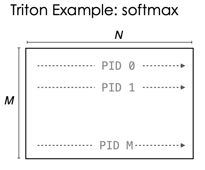
- each block is responsible for handling an entire row of the matrix
- each thread processes a single column within that row
- Instead of relying on separate primitive operations, which would introduce multiple memory read/write overheads, we utilize SRAM (shared memory) to store intermediate computations.
- All necessary operations (such as exponentiation, summation, and normalization) are performed in SRAM before writing the final results back to HBM
Template-based Graph Optimization
Graph Optimization: rewriting G to G’
- G’ run faster than G
- G’ output equivalent results
Template-based Graph Optimization: one of the most straightforward solution to do graph optimization.
- Engineers manually create (sub-)graph transformation(optimization) templates to guarantee both the correctness and the performance gain.
- Based on the templates, exhaustive pattern searching will be done over the dataflow graph and corresponding transformations will be applied.
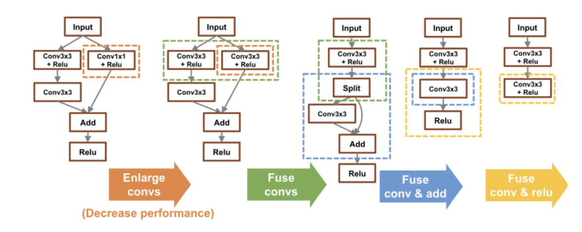
Fusion
combining multiple adjacent operators(operations) within a dataflow graph into a single, more efficient operation
Why Fusion improves performance?
- Reduce Kernel Launching
- Reduce I/O
Possible Downsides:
- Requiring Many Fused Operations:
FusedABCOp - At some point, codebase become unmanageable
CUDA Graph
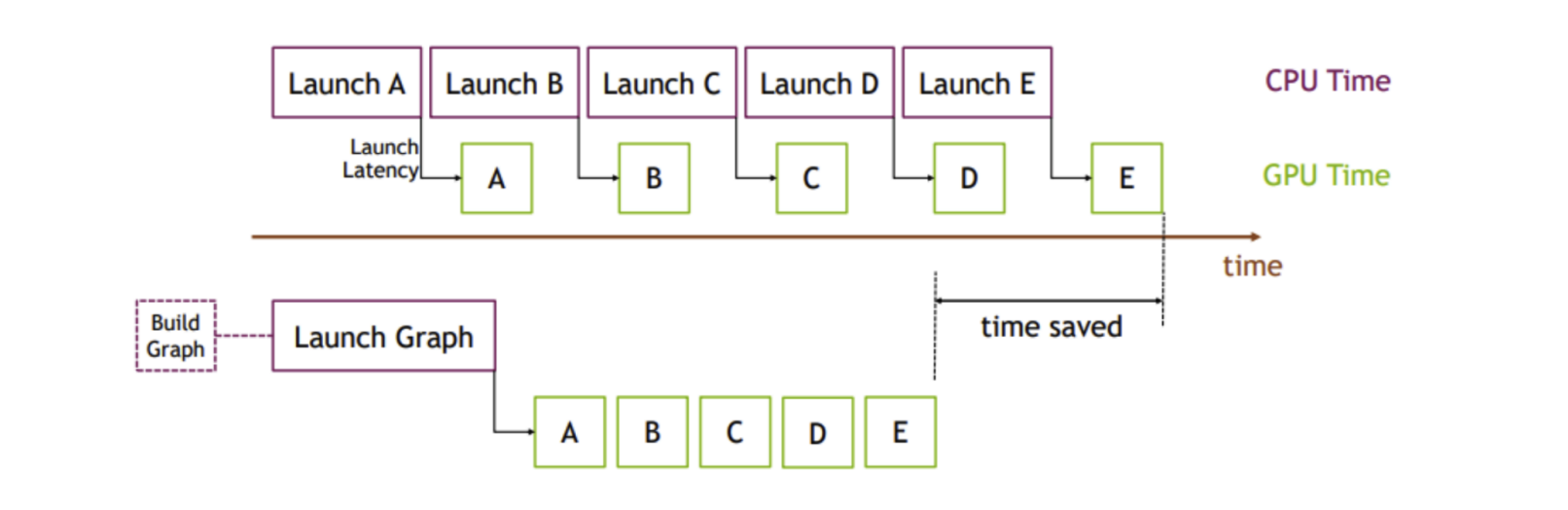
CUDA Graphs optimize the execution flow of entire operation sequences
- In traditional CUDA programming, CPU frequently sends commands to GPU to execute kernels, leading to overhead and latency
- CUDA Graphs will record the sequence of operations and execute them as a graph, reducing the overhead of CPU-GPU communication
Constant Folding
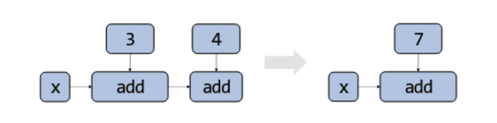
- Constant folding evaluates constant expressions at compile time
- Applying constant folding to a dataflow graph can reduce the number of operators or nodes
Common subexpression elimination
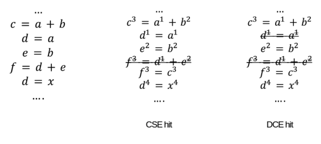
Example:
- Starting from the beginning of the code above, the value numbers are
{a: 1, b: 2, a+b: 3, c: 3, d: 1, e: 2, f: 3}. - At this point, we have a CSE hit since f has the same value number as a+b and c. To eliminate the redundant computation, we instead assign c to f.
CSE:
- compiler finds all occurrences of an expression and replaces it with a single instance holding the computed value
- assign unique value numbers to variables and expressions known to have same value at compile time.
Dead code elimination
Dead code elimination (DCE):
- removes code that is executed at runtime but whose result is never used again;
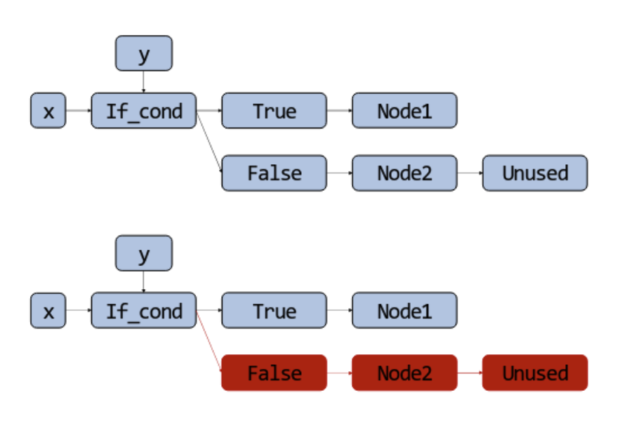
- if one direction of a conditional is never taken, the dataflow graph can be pruned
- if the false branch below is never used, we can remove the entire branch by traversing backward from the unused node.
Problem of Template-based Graph Optimization
- Greedy Template Matching Limits Performance Gains
- graph is constantly replaced with more efficient templates as they are matched by greedy algorithms
- might lose opportunities for global optimization
- To achieve higher performance gains, a larger search space is needed, allowing the optimizer to explore more complex transformations that may not be immediately beneficial but could lead to significant improvements in the long run.
- Scalability Issues Due to Variations in Graph Definitions
- variations in graph definitions across different ML operators, and graph architectures, and hardwares
- Each hardware backend (e.g., GPUs, TPUs) and each ML model architecture (e.g., ResNet, BERT) may require different optimization templates to achieve optimal performance
- for every combination of hardware, ML operators, and model architectures, human experts must manually design specific templates, and new operators and graph structures require more rules.
- labor-intensive approach
- Lack of Robustness and Guaranteed Performance
- The greedy heuristics of template matching and rules used by human experts to design templates are often specific to certain hardware or model architectures and may not generalize well to other configurations.
- performance gains from template-based optimizations are not guaranteed, as optimizations may miss subtle opportunities for performance improvements that are specific to certain DNNs or hardware backends.
Automate Graph Transformation
replacement for template-based graph optimization
TASO Workflow
a representative example of Automate Graph Transformation algorithm
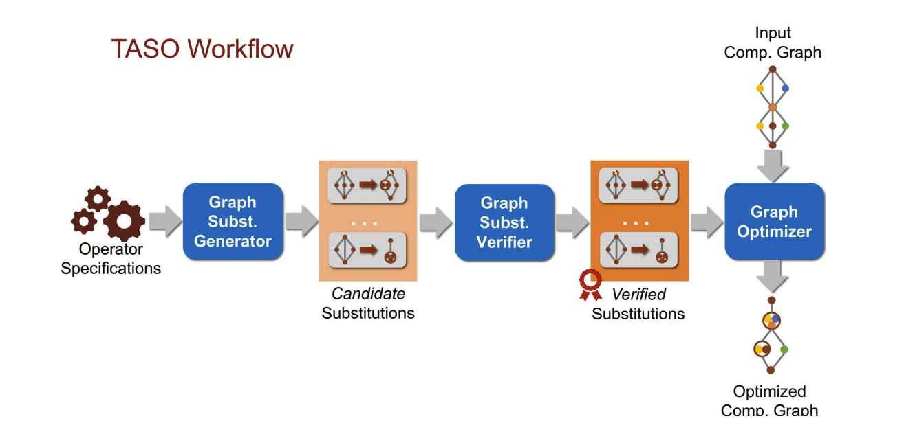
- Graph Substitution Generator:
- provides a dictionary of equivalent ML operator subgraphs
- key idea: find many set of ”equivalent subgraphs” that are easy to substitute like what we used to do in template-based approaches.
- To automatically generate such a dictionary:
- Enumerate all possible graphs up to a fixed size, which are composed by the ML operators
- Evaluate which ”pair” of graphs are equivalent – suitable for substitute.
- impossible to mathematically prove whether two graphs are equivalent
- give each of them the same random input and check if their outputs are the same
- Pruning Repeated Graphs: prune the substitutions using simple mathematical rules
- Variable Renaming: two graphs are equivalent if they differ only in variable names.
- Common Subgraph: the graphs differ only in the order of operations, A+(B×C) being equivalent to (B×C)+A
- Substitution Verifier:
- a formal verification method to ensure the correctness of the substitution in mathematical terms
- Define Specifications for Operators: Write down the mathematical properties and characteristics for each operator.
- P1: Convolution is distributive over concatenation.
- P2: Convolution is bilinear.
- Use an Automated Theorem Prover: Employ a compiler tool or automated theorem prover to determine whether two graphs are equivalent based on the mathematical specifications.
- Incorporating Substitutions: use trial-and-error approach to determine whether the substitution improves performance:
- selecting a verified substitution, matching patterns in the graph
- running the modified graph on a TPU to measure its performance
- By recording these performance results, a ‘Cost Model’ can be built: estimates the total computational cost by adding up the costs of individual operations
- To efficiently optimize the graph, the process involves traversing the graph, applying substitutions, calculating the cost, and using backtracking to refine the choices. This entire process is automated, removing the need for manually creating templates and performing pattern matching.
Summary for Graph Optimization
- workflow of graph optimization:
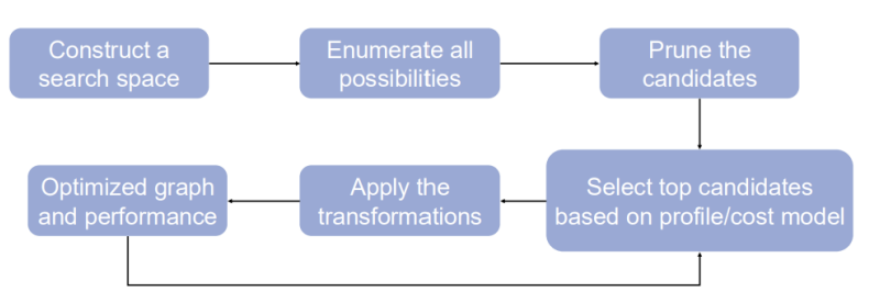
- a search space is created and all the possible combinations of operators are enumerated
- heuristics are used to filter out candidates that are either redundant or incorrect
- the best candidates are selected based on the Cost Model and transformations are applied to generate an optimized graph
- Once the graph is optimized and real performance data is collected, the Cost Model can be updated and refined
limitations
- The search space may not be large enough to include the best possible optimized graph. However, expanding the search space makes the process complex and time-consuming, creating a trade-off.
- The search process can be slow since it relies on trial and error method.
- Evaluating the resulting graph is expensive because real performance data is obtained after multiple iterations, which consumes GPU resources before improving the Cost Model.
Partially Equivalent Transformation (PET)
- FET: the fully equivalent transformation (FET) gives the same result as the original graph but it is missing some optimization opportunities.
- PET: partially equivalent transformation (PET) has better performance, but it gives a different result than the original graph
- solution: utilize the PET to improve the performance of the graph while maintaining the correctness of the output.
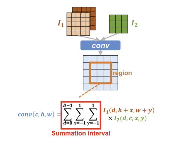
Example of conv2d PET
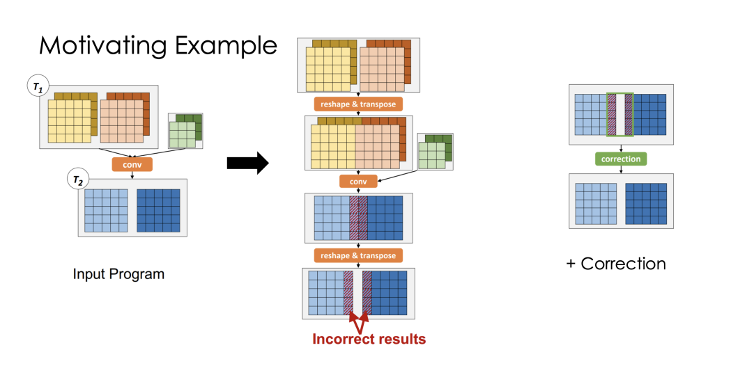
PET: concatenate the input matrices and apply the conv2d operation on the concatenated matrix
- Applying conv operation on a single matrix is 1.2 times faster than applying it on two matrices, since we are reducing kernel launches and memory I/O.
- Possible Workflow:
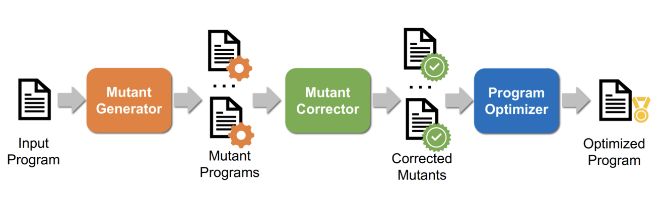
PET Workflow
- given an input program, we generate mutants, which are like substitutions but are not fully equivalent
- apply these mutants to the original program to get a faster version and then check if the mutated program’s results match the original program’s result
- If they do not match, we apply mutant corrector to correct the results.
- If added additional operators in the graph to correct the results, it will possibly increase the entire graph size. We will then manually fuse operators together to optimize the performance.
- Mutant Generator:
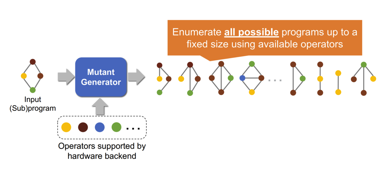
- generate mutant programs by enumerating all possible programs up to a fixed size using available operators
- Unlike substitution generators, we are not going to stop at just mathematically equivalent programs, instead we are going to enumerate partially equivalent programs as well.
- Detection and Correction the mutation results
- to check the result of original program and mutated program, the time complexity will be O(m x n), here m means number of possible inputs and n means output shape, to make things faster, reduce m and n:
- Reducing n:
- verifying the correctness of computations using only a small subset of outputs instead of evaluating the entire function.
- why works: neural network operations are largely multi-linear: output is linear with respect to each input,
(f(..., X + Y, ...) = f(..., X, ...) + f(..., Y, ...)), ` (f(…, aX, …) = a · f(…, X, …))` - Theorem: For two multi-linear functions f and g, if f = g for O(1) positions in a region, then f = g for all positions in the region.
- when apply conv operator, only need to check one position in one region, which largely reduce the computation costs from n to r (region number) and reduce O(mn) → O(mr), r (# regions) ≪ n
- here regions refer to the conv kernel size window on the input matrix
- Reducing m:
- Random testing
- If t random tests pass without detecting inequivalence, the likelihood of f and g being inequivalent becomes negligibly small. Random sampling replaces exhaustive enumeration with a probabilistic guarantee of equivalence, dramatically reducing computational cost.
- Reducing n:
- Correct the Mutant
- Recompute Incorrect Outputs Using the Original Program,serves as ground truth
- Identification of Errors: comparing the mutant program’s outputs with those from the original program, we can pinpoint the erroneous regions.
- Localized Correction: Instead of re-executing the entire program, only the specific incorrect regions are recomputed, significantly reducing the computational cost.
- Opportunistically Fuse Correction Kernels with Other Operators
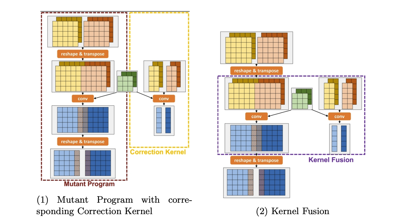
- To further reduce the overhead introduced by the correction process, kernel fusion is applied.
- reduce intermediate data movement
- Kernel fusion enables better utilization of hardware resources by executing correction operations alongside regular computations.
- Performance Optimization: The overall performance impact of error correction is mitigated, making the mutant program more efficient.
- Recompute Incorrect Outputs Using the Original Program,serves as ground truth
- to check the result of original program and mutated program, the time complexity will be O(m x n), here m means number of possible inputs and n means output shape, to make things faster, reduce m and n:
Workflow Review
| Aspect | Partially Equivalent Transformations | Graph Substitution |
|---|---|---|
| Core Idea | Explores a larger optimization space by allowing partially equivalent transformations that are not strictly mathematically equivalent but may achieve higher performance. | Focuses on generating and applying mathematically equivalent substitution rules based on strict operator specifications. |
| Components | 1. Mutant Generator: Enumerates all possible partially equivalent transformations using hardware-supported operators. 2. Mutant Corrector: Detects errors in mutant programs and corrects outputs with correction kernels and kernel fusion. 3. Program Optimizer: Further optimizes the corrected program for better performance |
1. Graph Subst.Generator: Generates substitution rules based on operator specifications and mathematical properties. 2. Graph Subst.Verifier: Ensures correctness of substitution rules via symbolic derivation and automated theorem proving. 3. Graph Optimizer: Applies validated substitution rules to optimize the computational graph. |
Memory
Batch Processing
| Term | Context | Meaning |
|---|---|---|
| Batch | Deep Learning | A group of training samples processed together |
| Mini-batch | Deep Learning | A smaller subset of a dataset used per training iteration |
| Micro-batch | Deep Learning | A split of a mini-batch for parallel processing |
| Batch Processing | Big Data | Processing large datasets in bulk |
| Micro-Batching | Big Data | Processing small groups of events in short time windows |
In deep learning, the terms batch, mini-batch, and micro-batch refer to different portions of the original training data being actively used:
- Batch: A group of training samples from the larger training dataset that are processed together.
- Mini-batch: A smaller subset of a batch, typically used in an iteration.
- Micro-batch: A further subdivision of a batch, used in pipeline parallelism.
In the context of big data, batch processing refers to the processing of a static subset of data, as opposed to an incoming stream of live data. Micro-batching, on the other hand, involves processing smaller groups of events within short time windows.
Memory and Scheduling
Totak Goal: peak memory during the execution is less than the available memory
peakMemory < availableMemory
Memory Consumption
When training models, the things that needed to be stored are:
- Model Weights
- Intermediate activation values: because in the backward pass, we need to derive the gradients using these.
- Optimizer States: because we do not always update weights by just gradients directly, but we do some computations on gradients, like applying Adam’s Optimizers etc. and then update the weights.
Determining Peak Memory
key questions to answer for determining peak memory:
- How large is the memory?
- What is the lifetime of the ‘memory needed’?
for every memory consumption component, we need two things: size and lifetime.
Lifetime for Inference Process
Basic Inference Process:
Primarily focus on the memory lifetime of weights and activations.
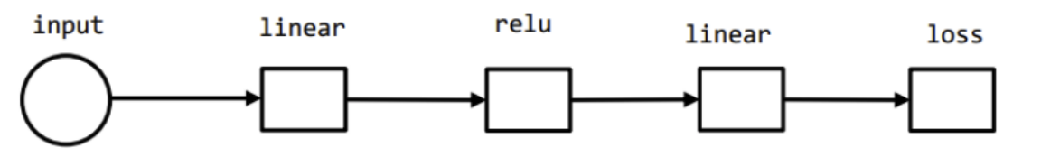
In a feedforward network, the computation at each layer follows a consistent pattern:
- Compute the weighted sum of the layer’s input.
- Apply the activation function to the weighted sum to obtain the layer’s output.
To minimize memory usage, we only need two memory buffers: one for storing the input of the layer, and the other to store the activated output.
In summary, memory of the model’s weights live throughout the inference process, while that of layer’s activation outputs are overwritten immediately as the next layer’s computation begins.
Size
Floating Point Standards
Common datatype for deep learning are:
- FP32 (4 Bytes each): 1-bit sign, 8-bit exponent, 23-bit mantissa
- FP16 (2 Bytes each): 1-bit sign, 5-bit exponent, 10-bit mantissa
- BFloat16 (also BF16, 2 Bytes each): 1-bit sign, 8-bit exponent, 7-bit mantissa
GPT3 Weight Size Estimation Example
A simplistic estimation of the parameter memory consumption of the full 175B GPT-3 is
175 billion × sizeof(a_parameter)
where each parameter can take up either 2 Bytes (16 bits) or 4 Bytes (32 bits). This means the memory space needed for the weights are 175 billion * 2 = 350GB or 175 billion * 4 = 700GB. A general rule of thumb for estimating model size: simply multiply the number of parameters with 2 or 4. Most models are stored in either 16- or 32-bit format.
Activation Size Estimation
convolution layer activation:
- batch size B, channel number C and spatial dimension H amd W
- B * C * H * W * sizeof(element)
multilayer perceptron (MLP) networks
- batch size B, output spatial dimension of M x P
- B * M * P * sizeof(element)
Transformer layer activation:
- Ignoring the inner working mechanisms of transformer attention blocks
- B * H * Lseq * sizeof(element)
With this we can revisit the full GPT-3 model, with batch size 3.2M and vector embedding dimension 12,288. Assuming a sequence length of 1, the number of elements of each transformer layer’s activation would be 3.2M * 12288 = 39.321B which considering each element taking 2 or 4 bytes, gives the total memory needed for the activation to be 78.64GB or 157.28GB.
Optimizer State Size (Adam)
Size The memory required to store the optimizer state for the Adam algorithm can be estimated as follows:
- Gradient with respect to parameters: N × sizeof(element)
- First moment: N × sizeof(element)
- Second moment: N × sizeof(element)
In total, the memory required for the Adam optimizer state is: Total Memory = 3N × sizeof(element)
Here, N represents the number of parameters in the model, and sizeof(element) is the size (in bytes) of a single parameter or gradient element (e.g., 4 bytes for a 32-bit float).
Lifetime for Training Process
In the context of training a neural network, tensors can be categorized as
- live tensors
- dead tensors
based on their usage during computation. Memory allocation is primarily required for live tensors.
Activation tensors are needed for both the forward and backward passes, especially in the backward pass where gradients are computed.
Training an N-layer neural network requires O(N) memory due to the need to store these intermediate activations. Optimization techniques can later be introduced to allow selective discarding of activations.
Memory overview for GPT-3
Note: Activation memory size is not accurate because transformers are composite layers.
- Model Parameters
- Parameters: 175B
- Precision: FP16/ FP32
- Memory: 175B × 2 bytes = 350 GB(FP16) or 175B × 4 bytes = 700 GB(FB32)
- Activations
- Layers: 96 (At Transformer Boundary)
- Precision: FP16/FP32
- Memory per Layer: 78 GB
- Total Memory: 96 × 78 GB = 7488 GB (FP16) or 96 × 156 GB = 14976 GB (FP32)
- Optimizer States
- Optimizer: Adam (first and second moments)
- Precision: FP32
- Memory per Parameter: 3 × 4 bytes = 12 bytes
- Total Memory: 3 × 175B × 4 bytes = 2100 GB
Memory Optimization Techniques
- Gradient Checkpointing (Activation Checkpointing): Selectively storing only a subset of activations and recomputing the rest during backpropagation.
- Gradient Accumulation: Training with large effective batch sizes while keeping per-step memory consumption low.
- CPU Swapping: Offloading data from GPU high-bandwidth memory (HBM) to CPU DRAM when needed.
Gradient Checkpointing
Key Idea: Instead of storing all intermediate activations, we can selectively store only a subset of them and recompute the rest during backpropagation.
Key Concepts:
- Forward Pass: The input is processed through multiple layers, generating activations.
- Backward Pass: The gradients are computed using the chain rule, requiring stored activations.
- Checkpointing: Instead of storing all activations, only a few are saved. The rest are recomputed when needed.
How it works:
- Divide the model into segments: Save only the activations at the boundaries of segments.
- Recompute Intermediate Activations: During backpropagation, recompute the activations for the layers between checkpoints as needed.
Using activation checkpointing introduces a trade-off:
- Memory Savings: Reduced memory usage by not storing every activation.
- Increased Computation: Additional computation is required to recompute activations.
Mathematical Model:
- For a network with N layers, if checkpoints are placed every K layers, the overall memory cost is approximated by:
- Memory Cost = O(N/K) + O(K)
- O(N/K): Memory for checkpoints
- O(K): Memory for recomputed activations between checkpoints
- The near-optimal trade-off is achieved when: K = √N
Pytorch Solution:
  import torch
  import torch.nn as nn
  import torch.utils.checkpoint as checkpoint

  class CheckpointedModel(nn.Module):
      def __init__(self):
          super().__init__()
          self.layer1 = nn.Linear(1024, 1024)
          self.layer2 = nn.Linear(1024, 1024)
          self.layer3 = nn.Linear(1024, 1024)

      def forward(self, x):
          x = checkpoint.checkpoint(self.layer1, x)
          x = checkpoint.checkpoint(self.layer2, x)
          x = checkpoint.checkpoint(self.layer3, x)
          return x
torch.utils.checkpointwill automatically discard the intermediate activations and recompute them during backpropagation.- Limitations: Only activations are checkpointed. The technique increases computation and may introduce numerical inconsistencies in stochastic layers.
Gradient Accumulation: Training with Large Effective Batch Sizes
Gradient accumulation allows training with a large effective batch size while keeping the per-iteration memory footprint small.
Concept:
- Compute gradients on several small mini-batches (micro-batches)
- Accumulate the gradients
- Perform a weight update after the accumulation, simulating a larger batch size
Mathematical Formulation:
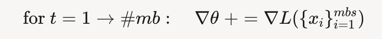
- split big batch into mini-batches:
#mb = mbs/bs - Before accumulation:
- After accumulation:
PyTorch Implementation:
```python
PyTorch Implementation:
```python
Without Gradient Accumulation
optimizer = … # 初始化优化器(如Adam/SGD) model = … # 定义模型 loss_fn = … # 定义损失函数(如CrossEntropyLoss) dataloader = …# 定义数据加载器
for epoch in range(…): # 遍历所有epoch for i, sample in enumerate(dataloader): # 遍历数据集 inputs, labels = sample # 解包数据
    # Forward Pass
    outputs = model(inputs)  # 前向传播

    # Compute Loss and Backpropagate
    loss = loss_fn(outputs, labels)  # 计算损失
    loss.backward()  # 反向传播

    # Update Parameters
    optimizer.step()      # 更新参数
    optimizer.zero_grad() # 清空梯度
With Gradient Accumulation
optimizer = … # 初始化优化器(如Adam/SGD) NUM_ACCUMULATION_STEPS = … # 梯度累积步数(模拟更大batch size)
for epoch in range(…): # 遍历所有epoch for idx, sample in enumerate(dataloader): # 遍历数据集 inputs, labels = sample # 解包数据
    # Forward Pass
    outputs = model(inputs)  # 前向传播

    # Compute Loss and Backpropagate
    loss = loss_fn(outputs, labels)  # 计算损失
    loss = loss / NUM_ACCUMULATION_STEPS  # 标准化梯度(模拟大batch)
    loss.backward()  # 反向传播(梯度累积)

    # 达到累积步数或数据集末尾时更新参数
    if (idx + 1) % NUM_ACCUMULATION_STEPS == 0 or (idx + 1 == len(dataloader)):
        optimizer.step()       # 参数更新
        optimizer.zero_grad()   # 清空累积梯度 ```
CPU Swapping
CPU swapping is a technique that offloads data from GPU memory (HBM) to the larger CPU DRAM
two primary operations:
- SwapOut: Moving activations or model weights from GPU VRAM to CPU DRAM.
- SwapIn: Retrieving data from CPU DRAM back to GPU VRAM when required for computation.
Mechanism in Deep Learning:
- In the forward pass, some activations may be swapped out to free up GPU memory
- In the backward pass, these activations are swapped back in before computing gradients.
When CPU Swapping is Effective
- It works well when computations are heavy, allowing data transfers to occur asynchronously.
- Suitable when swapped data is not needed immediately.
- Efficient when data transfer overhead is minimized through optimization.
Limitations and Challenges
- Frequent swapping may cause data transfer bottlenecks.
- Increased latency can slow down training, especially if the model is memory-bandwidth constrained.
- Not ideal for scenarios requiring constant, rapid access to the data.
Memory and Compute
Quantization
Key Concepts:
- Digital Representation of Data: Data is encoded into discrete values for digital processing.
- Basics of Quantization: Reduces precision to map continuous values to a discrete set.
- Quantization in ML: Lowers model precision to save memory and speed up inference.
- Post-Training Quantization: Converts trained models to lower precision after training.
- Quantization-Aware Training: Trains models while keeping check over quantization effects to preserve accuracy.
- Mixed Precision Training: Combines different precisions (e.g., FP16 & FP32) for efficiency
Post-Training Quantization
Quantization granularity:
- per-tensor: a single scale (S) and zero point (Z) are used to quantize an entire tensor, such as all the weights of a layer or all the activations in a layer
- simplest and most computationally efficient approach: requires fewer scaling factors and ensures the same precision for all weights
- may lead to a loss of accuracy, especially if the tensor contains large outlier weights or the range varies wildly across channels
- per-channel: where a separate scale (S) and zero point (Z) are assigned for each channel in a tensor
- for better preservation of numerical precision
- group: most fine-grained quantization method is group quantization where weights are divided into groups of elements and each group gets its own scale and zero point, such as quantizing per vector.
Multi-Level Quantization
Linear Quantization on Activations
Mix-Precision Training
Parallelization
Why develop large models?
- Enhanced Performance and Accuracy: Empirical evidence demonstrates that scaling models leads to improved performance across multiple benchmarks.
- Emergent Capabilities: Larger models exhibit emergent capabilities - newfound abilities that weren’t explicitly programmed but arise from the scale of the system.
Growing Challenge:
- Computational perspective: The gap between model growth and hardware capabilities is widening, as GPU and CPU advancement, still broadly following Moore’s Law, cannot match the exponential growth in model sizes.
- Memory perspective: The memory requirements of large models are outpacing the available memory on GPUs, leading to memory bottlenecks.
Types of parallelism
- Data Parallelism: Distributing data across multiple devices and performing the same computation on each subset of data.
- accelerator level: SIMD
- GPU level: distributing data across numerous cores, with each core handling a portion of the computation.
- across multiple GPUs: each device processes a subset of the data.
- Core Assumption: the whole model fits on a single GPU
- Model Parallelism: If the model does not fit on a single machine, we must adopt model parallelism.
- model perspective: model is basically a computational graph, involving many ’MATMUL’ and non-linear functions
- How we partition a model is equivalent to thinking about how we partition tensor operators.
- Intuitive Example:
- cut in the middle by feeding the first few layers of the model to a single GPU and the next remaining layers to another GPU
- pipeline the execution to make it more efficient
- or cut horizontally instead of vertically
Computational and system perspective
- Computational Side:
- parallelize by partitioning the compute function across different GPUs
- optimizer f, where we optimize gradients to parameters. We apply function f across different GPUS
- memory Side:
- D, the data or the number of batches we need to partition D
- θ, wherein we partition the parameters
communication challenge
Handling communication parameters and activations depends on the NN graph partitions
Parallelism workflow
In data parallelism, the parameters and model code are replicated across the GPUs, and they perform the respective computation on the specifically designated batch of data. They will produce copies of gradients. These gradients need to be synchronized. All GPUs’ gradients have to be accumulated and applied to parameters. This generates a new copy of parameters, which then need to be redistributed across the GPUs.
In model parallelism, we partition the model. Either partition the model parameters (θ) or partition the gradient (∇l) computation function. We need to figure out how to deal with data (partition or not partition). Further, we need to partition the optimizer states.
Parallelism in action
parallelization can be treated as partitioning of a computational graph (forward, backward, and weight update graphs) on a device cluster by being subject to memory constraints and communication bandwidth.
- fast connections within node: nvlink
- slow connections between nodes
problem definition:
After partitioning, we want it to be as fast as possible without additional memory.
Intra and Inter parallelisms
Communication Characteristics
Here op means an operator, might be something more complex than a single operator, like a subgraph.
- Inter-op parallelism
- Assign different operators to different devices. The second op depends on the output of the first op.
- Typically requires point-to-point communication between consecutive operators (e.g., sending outputs from Device 1 to Device 2).
- Potential device idle time when an operator finishes early and must wait for other operators to complete their tasks before proceeding to the next stage.
- Intra-op parallelism:
- Splits a single operator across multiple devices (e.g., large matrix multiplication).
- Typically relies on collective communication (all-reduce, all-gather, broadcast, etc.) to merge partial results.
- High throughput when well-implemented, but communication overhead can be significant if the operator is not large enough or if the network is slow.
Example
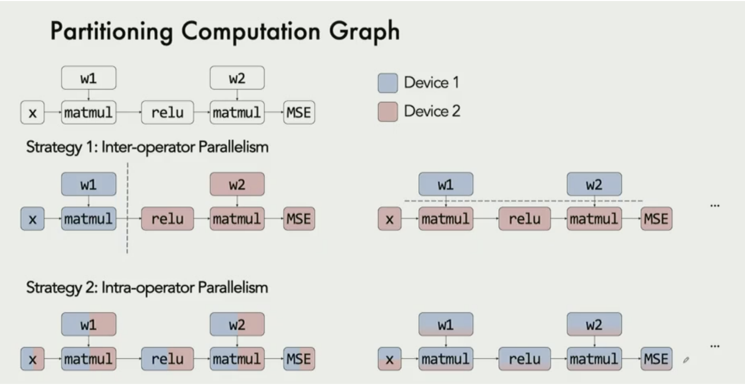
possible partition strategies:
- Inter-Operator Parallelism:
- device 1 takes the first matmul layer, while device 2 takes the remaining layers
- or do a horizontal cut, where device 1 takes the w1 and w2 and putting the rest on device 2
- Intra-Operator Parallelism:
- cutting the operators, the weights, the input, and outputs half and half, sharing among two devices. (Both horizontally and vertically)
Question: Is data parallelism intra or inter parallelism? Answer: It is intraparallelism.
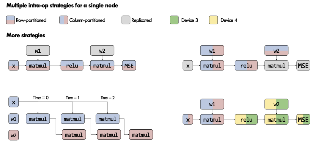
intra-op strategies for a single node:
- Row-partitioning:
- The input matrix is partitioned by rows, each partition (shown in blue/red) processes different rows of the input, operations like matmul are performed on these row partitions independently
- Model-partitioning (Megatron), like the forth graph in the previous image:
- a hybrid of model and tensor parallelism with the workload is split across different devices.
- Each colored section (blue/red) represents different parts of the model running on different devices, Operations like matmul and relu are distributed across devices.
- Pipeline parallelism:
- A way for temporal parallelism, operations are executed in a staged manner across time (Time = 0, 1, 2), different parts of the model (w1, w2) work on different timesteps, Enables better hardware utilization through pipelined execution.
Trade-offs
- Inter-op parallelism:
- simple to implement
- idle time
- synchronization bottleneck
- P2P communication
- Intra-op parallelism:
- deliver high speedups for computationally heavy operators (like large matrix multiplications), but collective communication steps can become bottlenecks.
- collective communication operation like all-reduce is very costy, so the intra operation parallelise is better to be adapt to data cluster that gots higher innter bandwith.
- optimal parallelism strategy often involves a hybrid approach
to be more specific:
Benefits of Inter-Op parallelism include:
- Parallel Execution of Independent Operations: Different operations (nodes) in the computational graph that have no dependencies are executed simultaneously on different devices.
- Graph-Level Parallelism: Focuses on scheduling tasks from the computational graph across multiple devices, improving overall throughput.
- Efficient for Multi-GPU Systems: Allows better utilization of all available hardware resources by distributing independent tasks.
- Reduces Latency for Complex Graphs: This type of parallelism performs well when models have multiple parallel and independent sub-graphs. Thus, it is especially useful for neural networks with multiple branches or parallel components (e.g., ResNet, Inception models).
- Examples: TensorFlow’s XLA Compiler and optimized task schedulers for deep learning frameworks.
Some trade-offs of this approach include:
- Device Idling: This use of P2P communication can result in some devices idling while they wait for others to complete.
- Device Communication: On the other hand, this approach results in less device communication than Intra-Op parallelism, avoiding this pitfall.
Some benefits of Intra-Op parallelism include:
- Parallel Execution Within a Single Operation: Large operations, such as matrix multiplications or convolution layers, are parallelized across multiple devices.
- Focus on Single Task Acceleration: Optimizes the execution of individual operations to reduce their runtime.
- Tensor Partitioning and Sharding: Splits large tensors across multiple devices for simultaneous computation.
- Applicable for Large-Scale Linear Algebra Operations: Particularly beneficial in deep learning models with large parameter matrices.
- Device Utilization: This approach results in high device utilization as each device will generally have a part of an operator to work on.
- Examples: CUDA-based parallelism for matrix operations, MKL-DNN, and cuDNN optimizations.
Model Flops Utilization (MFU)
How to measure the efficiency of parallelism?
- Arithmetic Intensity (AI) is usually an effective metric for single operator level
MFU(model flops utilization):
MFU = (#Flops/t) / peakFLOPS#FLOPs: Total floating−point operations performed by the ML programt: Time taken to complete the program-
peakFLOPS: The maximum theoretical FLOPs the hardware can perform - MFU performs the calculation by considering the workload of the computation as well as the hardware’s capabilities.
- MFU values close to the peak FLOPS can only be achieved if we use only GEMM operations and almost no MFU-unfriendly operations.
- GEMM: General Matrix Multiplication
Potential Factors Affecting MFU
- Op Types in the Computational Graph: The type and shape of operations in the ML model can affect MFU. For example, Different operations (e.g., matrix multiplication, convolution) have different FLOPs which can affect MFU.
- Precision, Core, and GPU Type: The hardware’s precision (e.g., FP32, FP16), core count, and GPU type (e.g., V100, A100, H100)influence peak FLOPs and thus MFU.
- Communication Over Network: Network communication can introduce delays, reducing MFU.
- Optimizations:Poorly optimized code or inefficient use of hardware resources can lower MFU. Techniques like precision reduction, core utilization,memory-efficient kernels, better scheduling and GPU type selection can impact MFU.
MFU-Friendly and MFU-Unfriendly Operations
- MFU-friendly operations: Operations that maximize FLOPs utilization, such as matrix multiplications (matmul) with high arithmetic intensity.
- MFU-unfriendly operations: Operations that involve more data movement or memory-bound than computation, such as element-wise operations (e.g., ReLU) or data shuffling.
Reducing Communication Overhead Techniques like overlapping computation with communication (e.g., using asynchronous communication) or optimizing data transfer (e.g., reducing message size) can help reduce or hide communication overhead.
MFU Estimation
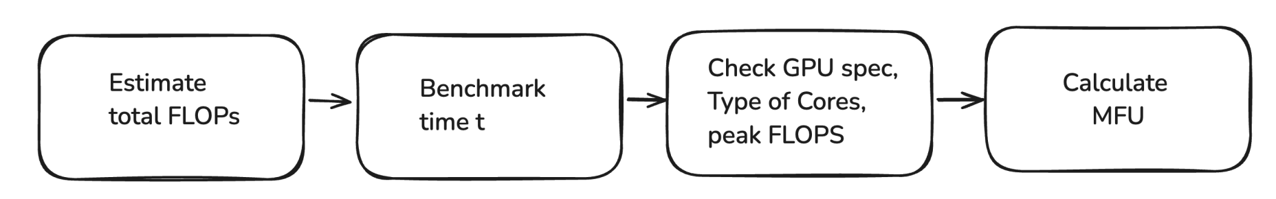
Suppose:
- #FLOPs = 10^12 (1 trillion FLOPs).
- t = 10 seconds.
- peakFLOPS = 10^13 (10 trillion FLOPs per second).
The MFU is calculated as:
MFU = (10^12/10) / 1013 = 0.01 or 1%
This means the hardware is only 1% utilized, indicating it is underutilized and must be optimized further.
MFU comparing to HFU
| MFU | HFU |
|---|---|
| MFU measures how efficiently the model uses the hardware’s computational capacity | HFU measures the actual utilization of hardware’s peak performance, considering all active processes and overheads. |
MFU = EstimatedAchievedFLOPs / PeakTheoreticalFLOPS |
HFU = ActualAchievedFLOPs / PeakTheoreticalFLOPS |
MFU (Model Flop Utilization) and HFU (Hardware Flop Utilization) are typically assumed to be equal. However, when using certain memory-saving techniques like gradient checkpointing, this assumption no longer holds. There can also be some overhead beyond the pure model computation. Gradient checkpointing reduces memory usage by recomputing intermediate activations during backpropagation. While this saves memory, it introduces additional computations that do not directly contribute to model convergence. As a result, HFU can appear higher than MFU in such scenarios.
The computation calculations are as follows:
Without Checkpointing:
- Forward Pass: 1 pass
- Backward Pass: 1 pass
- Total Equivalent Forward Passes: In most neural network models, a backward pass involves approximately twice the computation of a forward pass because it involves the calculation of gradients with respect to both parameters and activations. Therefore, 1 backward pass ≈ 2 forward passes. Total: 1 (forward) + 2 (backward) = 3 forward passes
With Checkpointing:
- Forward Passes: 2 passes (an extra pass is required for checkpointing to recompute certain activations needed for the backward pass, as not all activations are stored)
- Backward Pass: 1 pass
- Total Equivalent Forward Passes: Using the same equivalence, 1 backward pass ≈ 2 forward passes . Total: 2 (forward) + 2 (backward) = 4 forward passes
Comparing MFU and HFU:
- Without checkpointing, the total is 3 forward passes.
- With checkpointing, the total increases to 4 forward passes.
- This relationship can be expressed as:
MFU = 3/4 * HFU
Collective Communication
Collective communication is a type of communication that involves multiple processes or devices working together to exchange data. It is commonly used in distributed computing and parallel processing environments, where multiple devices need to share information efficiently.
- Broadcast
- In broadcast, data from a single process/rank is distributed to all other processes in the group
- Reduce
- combine values from all processes and assign the result to a single process
- commonly used for summation, product, or finding minimum/maximum
- Broadcast and Reduce-to-One can be thought of as inverse operations, although not in a mathematical sense, since the aggregations performed in reduce are often irreversible.
- Scatter
- Splits data from the array in a single rank into equal-sized chunks, and sends each chunk to a different process.
- Each process gets a unique portion of the data.
- Gather
- Gather can be thought of as the inverse of scatter.
- Each process has a portion of an array, and scatter collects data from multiple processes and combines it into a single process in a structured way.
- Allgather
- An extension of gather
- every process collects and shares data from all other processes
- Instead of sending all the data to a single target process like gather does, the collected data is sent to every process.
- Reduce-scatter
- Combines reduce and scatter operations.
- First, each process contributes a data chunk, and an element-wise reduction (e.g., sum, min, max) is applied across corresponding chunks from all processes
- Then, instead of keeping the full reduced result, each process receives only a unique portion of the reduced data (the scatter process).
- Allreduce
- Combines reduce and broadcast operations by reducing data to a single result and broadcasting it back to all processes.
Facts
- Collective communication is significantly more expensive than point-to-point (P2P) communication. In collective communication, we ask all our ranks to communicate, compared to just two in p2p.
- Collective operations can be constructed using multiple P2P communications.
- Look out for “X”CCL libraries such as NCCL, MCCL, and OneCCL for optimized implementations. The strength of Nvidia’s NCCL library is part of the reason behind their recent success.
- Collective communication is not fault-tolerant, and failure in one process may disrupt the entire operation.
Communication Model
rough model:
α + nβ, β =1/B
- α is the initial cost of setting up connection
- β represents the inverse bandwidth
- n is the message size
- Small Message Size (α » nβ): Latency (α) dominates; the focus is on reducing communication latency.
- Large Message Size (α « nβ): Bandwidth utilization (nβ) dominates; the focus is on maximizing bandwidth.
There are two families of algorithms to implement the collective communication primitives.
- Minimum Spanning Tree Algorithm for small messages.
- Constructs a spanning tree connectivity, so that the overall cost has the minimum number of α.
- like Prim, Kruskal
- Ring Algorithm for large messages.
- Each process communicates with its neighbor in a ring-like structure, ensuring full utilization of device parallel and bandwidth.
MST in Operations: Small Model
Minimum Spanning Tree (MST) algorithm plays a crucial role in communication models that prioritize low latency.
- MST approach assumes a network where each node can communicate with only one other node at a time.
- Unlike approaches that aim to maximize throughput by utilizing all available links, MST selectively engages connections to reduce latency.
- As a result, many network links remain idle, and bandwidth is not fully leveraged.
- this trade-off is intentional, as MST is designed to minimize initial communication delay rather than optimize overall throughput.
Characteristics and Trade-offs
- minimizing latency comes at the cost of bandwidth efficiency. Since each node only communicates with a designated target node, many potential communication links remain unused, leading to a scenario where bandwidth resources are underutilized.
- One of the fundamental principles of MST-based communication is its ability to break down complex reduction operations into more manageable components.
- MST achieves this by dividing the reduction process into smaller, more manageable steps, allowing for efficient and concurrent execution.
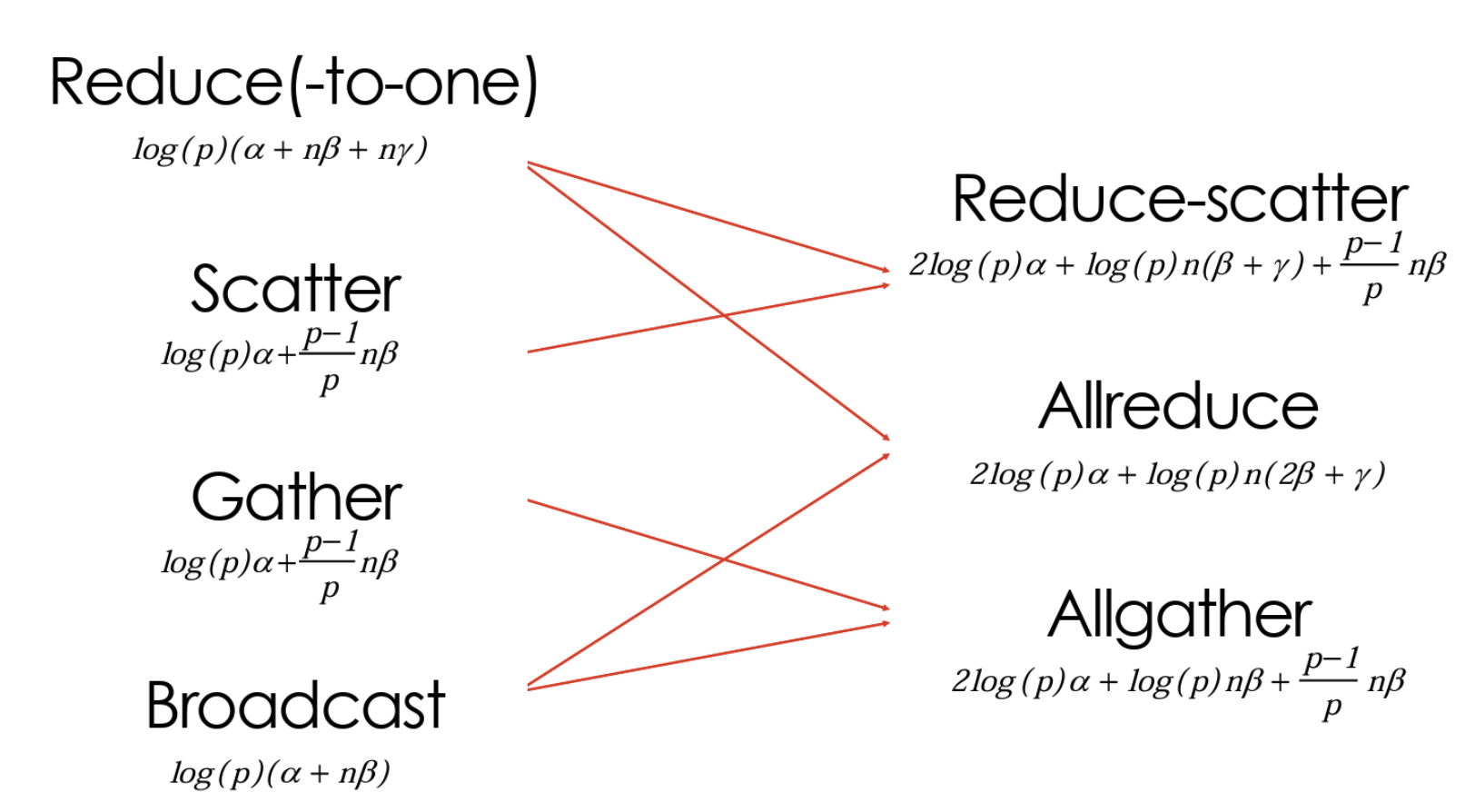
- here
pis the number of processes,γis the time taken for other factors like computation
Ring Algo in Operations: Large Messages
Key Characteristics
- Uses Links Between Every Two Nodes → Ensures full bandwidth utilization.
- Higher Latency; Number of Rounds Doesn’t Matter → Prioritizes bandwidth over minimizing communication rounds.
- Logical Ring in a Physical Linear Array → Uses worm-hole routing to avoid conflicts in wraparound messages.
- worm-hole routing: a technique that allows messages to be sent in smaller segments, and also enables nodes to receive and forward messages without waiting for the entire message to arrive, forming a continuous flow of data.
How It Works
- Message Splitting : A large message is divided into equal-sized chunks. For a message of size n, each of the p nodes gets n/p data.
- Sequential Data Transfer:
- Each node sends a chunk to the next node while receiving a chunk from the previous node.
- This ensures continuous data transfer and prevents idle nodes.
- Full Utilization of Links:
- All available bandwidth is used as each node is actively engaged in sending and receiving.
- Unlike MST algorithms, no links remain underutilized or idle.
Advantages Over MST
- Bandwidth Optimality → Unlike MST, where some links are idle, Ring Algorithm ensures all links are utilized.
- Scalability → Works efficiently for arbitrary numbers of nodes.
- Better Performance for Large Messages → Since the algorithm focuses on bandwidth rather than latency, it performs better when message sizes are large.
Example: AllReduce
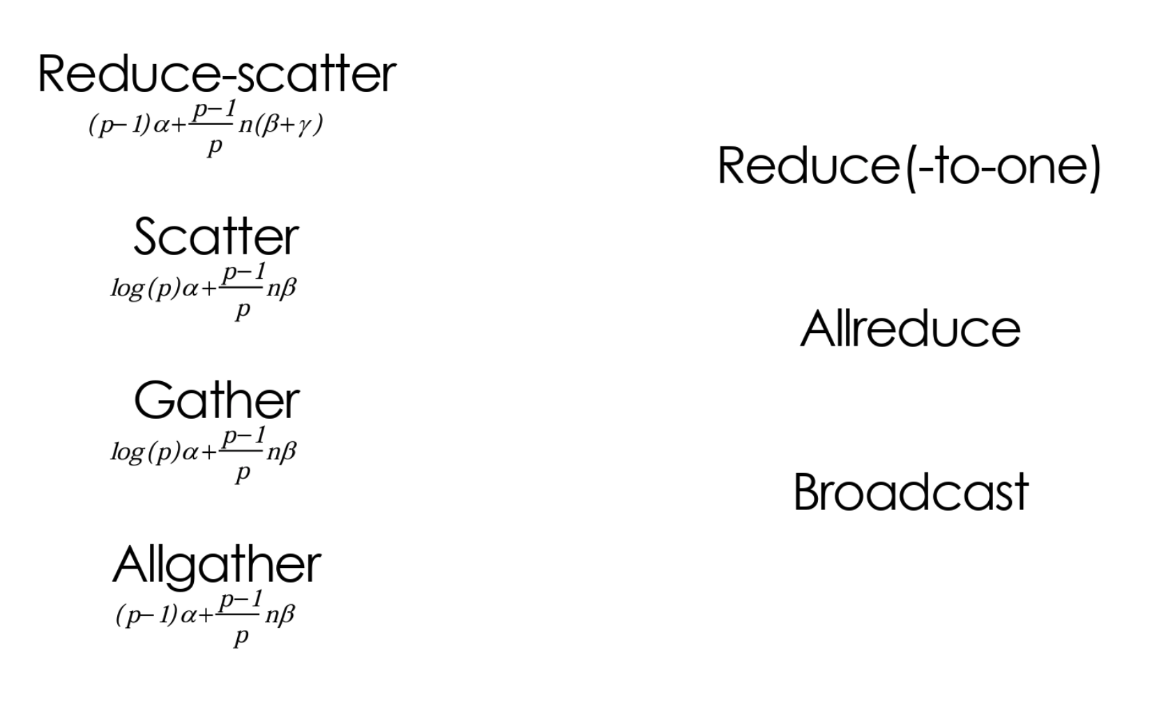
Data Parallelism
Communication Challenge
For Common Data Parallelism, input data is partitioned across multiple computing devices. Each device maintains a local copy of the model parameters and processes a different subset of the data.
- During the forward pass, computations occur independently on each device without requiring communication.
- In the backward pass, each device computes gradients based on its assigned batch, resulting in partial gradients that are local to each device.
- challenge arises because updating the model correctly requires each device to access the full gradient information from all devices.
Two solutions:
- Parameter Server Approach
- All-Reduce Approach
The above two approaches have a basic assumption that the model fits on a single gpu worker.
Parameter Server Approach
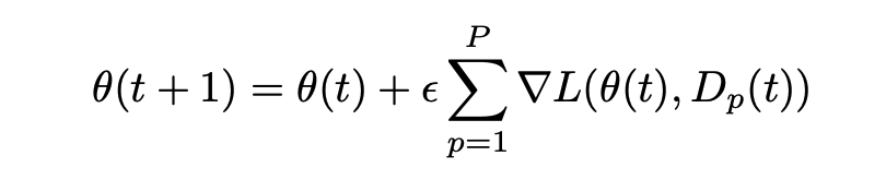
- P is the number of workers
- In this approach, each worker independently computes gradients without any communication during this step.
- Once the gradients are computed, all workers send them to the central parameter server.
- The server aggregates the received gradients, updates the model parameters accordingly, and then sends the updated parameters back to all workers. This ensures that every worker uses the same model in the next iteration.
Two main assumptions underlying this approach:
- each iteration involves heavy communication overhead, as all workers must continuously exchange data with the central server.
- in the era of 2012, the compute-to-communication ratio was approximately 1:10, meaning that communication costs were significantly higher compared to computation.
Two main challenges:
- communication bottleneck—since all workers must send gradients to and receive updated parameters from the same server, scalability becomes a critical issue.
- single point of failure—if the parameter server crashes, the entire training process is disrupted.
Server bottleneck
Example: All-Reduce
- each worker send that shard of gradients to the server that holds the shard
- send new model parameters back to the workers
Syncronization operations here:
- Every time each worker finishes the gradient, it has to send the gradient to the server, server aggregate that and send it back.
- overall speed is limited by the slowest worker.
Consistency Models for Parameter Server
BSP (Bulk Synchronous Parallel): box synchronous consistency
- periodically synchronize the model parameters between every worker
- might cause bubbles
- top level synchronization
Relaxed Consistency: Using Server as a Gradient Aggregator
- To reduce bubbles, we can relax the box synchronous consistency
- intuition: each worker computes a copy of gradients, and the server aggregates these gradients before performing gradient descent.
- machine learning algorithms are highly error-tolerant, meaning that even with some introduced errors the model can still function effectively, we can allow some deviation without compromising convergence.
- can use a ”slightly wrong version” of the gradients to update parameters under certain conditions
Relaxed Consistency: Asynchronous Communication (ASP, No Consistency)
ASP: Asynchronous Parallel
- no barrier, no synchronization, no aggregation
- not working
Relaxed Consistency: Bounded Consistency (SSP)
SSP: Staleness Synchronous Parallel
- allows workers to use a slightly outdated version of the model parameters
- set a staleness bound (S) to limit the maximum allowed staleness of the model parameters
- staleness variable impacts whether the model converges or not:
- if S is too large, the model may not converge
- if S is too small, the model may not fully utilize the available compute resources
- Faster worker will be blocked in order to limit the staleness of the model parameters
SSP Expectation Bound
- upper bound for the difference between a staleness estimate and true estimate exists
- check “SSP Expectation Bound Equation” for more details
AllReduce Approach
The most popular AllReduce interface is DDP(Distributed Data Parallel), provided by PyTorch.
- In DDP, we declare ranks among all the processes and then for each rank a duplicated model will be declared.
- based on the ring algorithm, each rank will send its gradients to the next rank and receive the gradients from the previous rank.
- first reduce than broadcast
- The weakness of AllReduce is that it is not fault tolerant. If one worker fails, the whole AllReduce will fail.
From Computational Graph (Neural Networks) to Stages
For better inter-parallelism, whole computational graph is divided into stages
- model is too large to fit on a single GPU
- stages are operated in a sequential manner
- The data transfer between stages is small because only the outputs are being transferred.
pipeline bubbles:
bubble_area / total_areacalculates bubble percentage
Reduce Bubbles
pipelining inputs
- With pipelining inputs, bubble percentage becomes
(D - 1) / (D - 1 + N)- D devices and N inputs
- This only works for the inference stage because each computation is independent of others.
- At training stage, layer dependency is introduced by back propagation, such waiting may introduce more bubbles.
Possible Solutions for Reduce Training Bubbles:
- Device Placement: Ensure that each stage in the pipeline has a similar computation time to prevent idle time in certain stages.
- Synchronous Pipeline Parallel Algorithms: Introducing strong consistency by providing stable training but have bubbles due to synchronization. (GPipe, 1F1B and Chimera).
- Asynchronous Pipeline Parallel Algorithms: Introducing relax consistency by reducing bubbles but introduce stale gradients, which may impact model convergence. (AMPNet, Pipedream/Pipedream2BW)
Synchronous Pipeline Parallel Schedule
Synchronous pipeline parallel schedule aims to enhance efficiency by modifying the pipeline execution strategy while preserving the exact computation and convergence semantics as if training were conducted on a single device.
- This approach ensures that parallel execution does not introduce inconsistencies in gradient updates or training dynamics.
GPipe
GPipe is a pipeline parallelism approach that partitions the input batch into multiple micro-batches and processes them sequentially across different devices.
- Instead of waiting for the full batch to complete before starting the backward pass, GPipe enables overlapping computation by pipelining the forward and backward passes of different micro-batches.
- The gradients from each micro-batch are accumulated, ensuring that the final parameter update is equivalent to training with a single batch
Disccusion about number of micro-batches:
- The proportion of pipeline bubbles:
D - 1 / (D - 1 + N) - The number of micro-batches (N):
- bigger N leads to better utilization of the pipeline
- bigger N reduces the size of each micro-batch, which can negatively impact computational efficiency. A smaller micro-batch leads to lower arithmetic intensity, reducing the device utilization due to inefficient memory access patterns and increased CPU overhead.
- Memory consumption per device:
memory usage = Parameters + Activations * numnber of micro-batches- increasing the number of micro-batches raises memory consumption. The number of micro-batches is therefore constrained by the available memory on each device.
1F1B
1F1B schedule is an optimization to the GPipe schedule that reduces memory usage through more efficiently scheduling backwards calculations.
- 1F1B schedule prioritizes the execution of the backwards pass, meaning as soon as there becomes a microbatch available for the backwards pass, it is then processed.
- 1F1B schedule has the same latency as the GPipe schedule, but where the optimizations come in is that it allows for memory to be realeased earlier.
- The 1F1B method uses less memory, and only needs to store the number of devices rather than the number of microbatches. It is the method that is adopted today for training GPTs and LLMs.
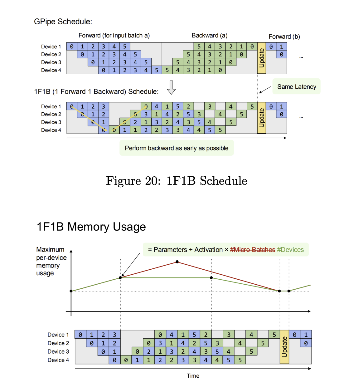
Interleaved 1F1B Schedule
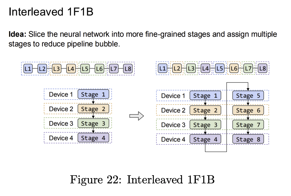
A further optimization of the 1F1B schedule is the interleaved 1F1B method
- Here, the neural network is sliced into finer stages and each device has multiple stages
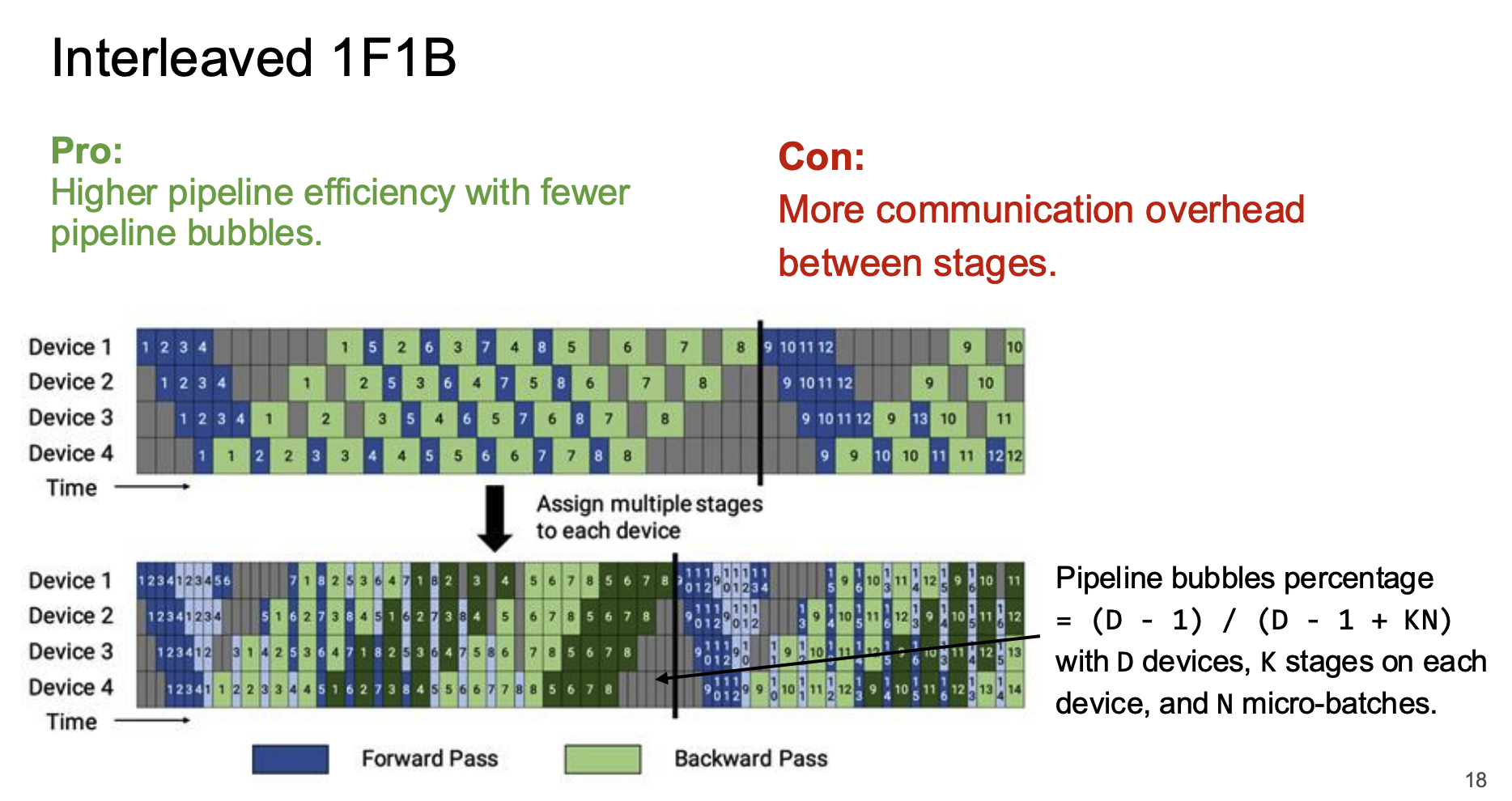
The new schedule further reduces the pipeline bubble. Whereas the regular 1F1B method had the same latency as GPipe, the interleaved 1F1B schedule reduces latency.
The cost of this is that since there are more stages there is a more communication between devices, adding additional communication overhead. However, the communication cost is generally small so the method is overall more efficient.
Terapipe & Chimera
Terapipe is pipeline parallelism for autoregressive models (GPT, Transformers).
- The key insight here is that the next token only depends on previous tokens, so we can put each layer on a device and pipeline
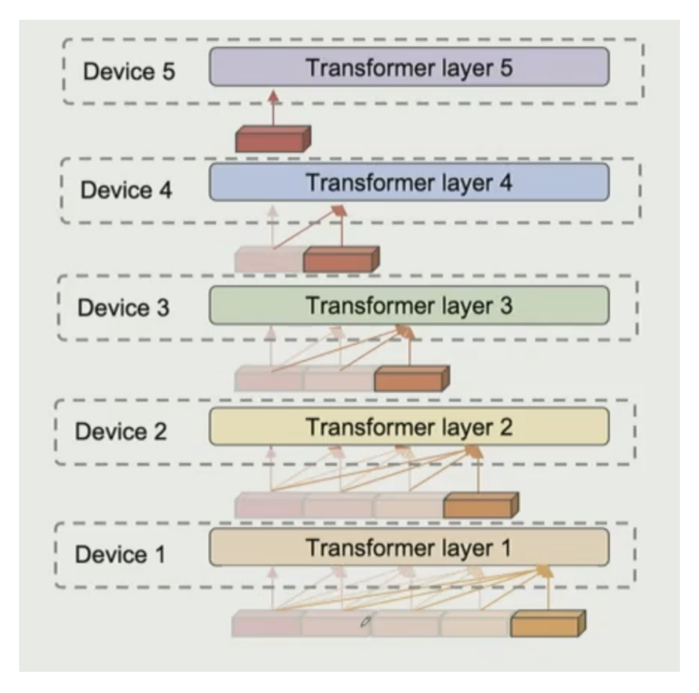
Chimera is the pipeline parallelism used in Deepseek. It attempts to further optimize the 1F1B pipeline by having one set of batches go in the opposite direction on the devices as the image below shows.
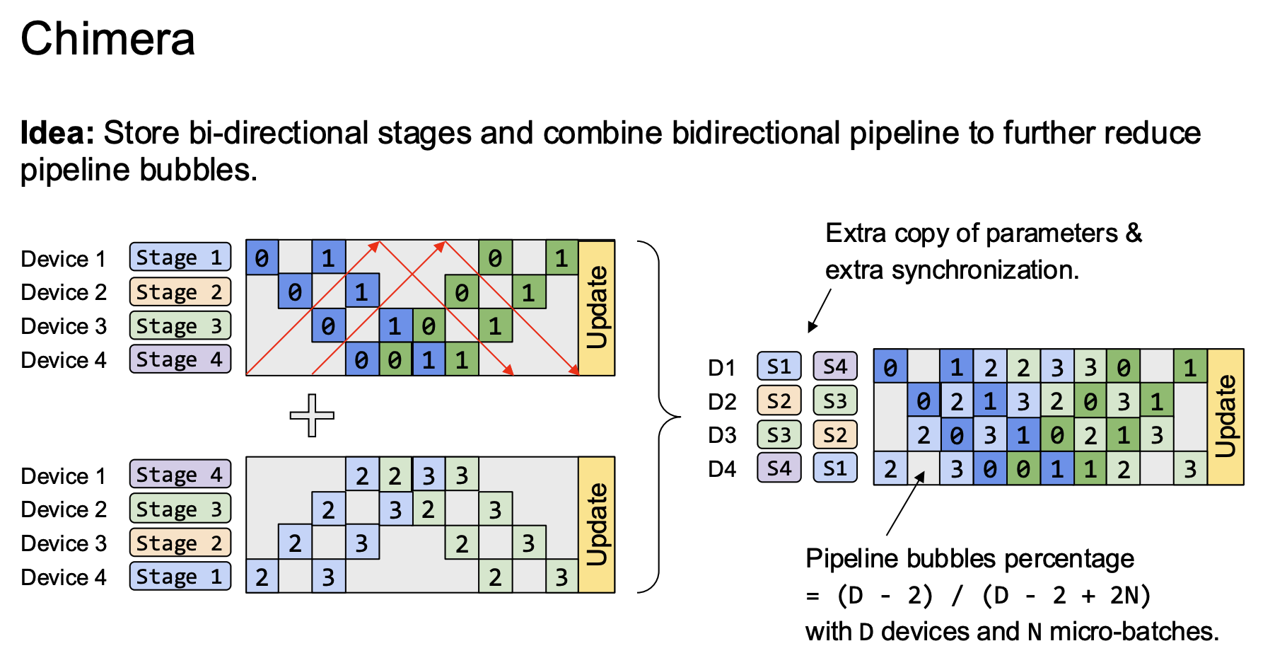
Synchronous Pipeline Schedule Summary
- Pros: Keep the convergence semantics. The training process is exactly the same as training the neural network on a single device.
- Cons: Pipeline bubbles. Reducing pipeline bubbles typically requires splitting inputs into smaller components, but too small input to the neural network will reduce the hardware efficiency.
Asynchronous Pipeline Schedules
- Remove the synchronization point in the pipeline schedule
-
start the next round of forward pass before backward pass of the previous round finishes
- Pros: No Pipeline bubbles.
- Cons: Break the synchronous training semantics. Now the training will involve stalled gradient. Algorithms may store multiple versions of model weights for consistency.
AMPNet
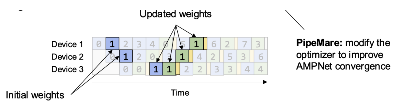
Idea: Fully asynchronous. Each device performs forward pass whenever free and updates the weights after every backward pass.
- With this schedule, the different stages in the forward and backward pass can be on different versions of the weights because each device update on their own pace.
- For example, for data 1, the forward pass in stages 1 and 2 still uses the initial weights (blue 1), but during the backward pass, its gradient updates are based on the weights modified after training with data 0 (green 1).
- weight staleness introduces noise, affecting training convergence.
- PipeMare alleviates this issue by optimizing the optimizer strategy
Convergence: Achieve similar accuracy on small datasets (MNIST 97%), hard to generalize to larger datasets.
PipeMare improve the convergence of AMPNet: It modifies the gradient optimizer to improve the convergence a little bit. But it cannot foundamentally changed the drawback of this way.
Pipedream
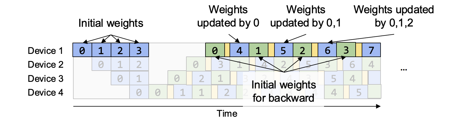
Pipedream improves the convergence by reducing the asynchronous staleness
- update the model’s weights once the backward has finished.
- Enforce the same version of weight for a single input batch by storing multiple weight versions.
Detailed explanation for the given image:
- During the forward and backward passes for input batches 0 to 3, the same initial weights are used.
- for input batch 4, the forward pass utilizes weights that have been updated by input batch 0.
- Since the backward pass for input batches 1 to 3 still requires the initial weights, at this point, two copies of weights exist:
- Initial weights (for the backward pass of input batches 1 to 3).
- Weights updated after processing input batch 0 (for the forward pass of input batch 4).
Similarly, for input batch 5, weights updated by input batches 0 and 1 are needed. For input batch 6, weights updated by 0, 1, and 2 are required.
As a result, we need to store four copies of weights in total. However, since the neural network is divided into only four stages, no memory is saved, defeating the purpose of pipeline parallelism in terms of memory efficiency.
- Convergence: Similar accuracy on ImageNet with a 5x speedup compared to data parallel.
- Con: No memory saving compared to single device case.
Pipedream-2BW
To reduce the memory usage, the authors of Pipedream proposed a modification to the original pipeline by updating the weights less frequently
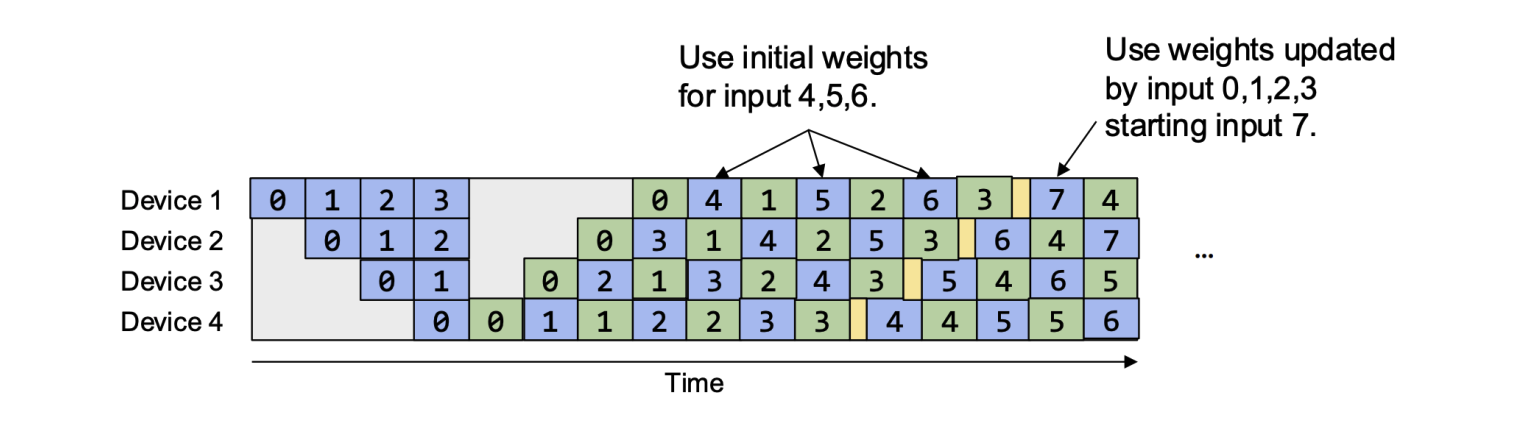
for input batches 4, 5, and 6, the initial weights are still used. Starting from input batch 7, the model begins using weights updated by input batches 0 to 3.
This means that the green weights (updated weights) are only stored for one update cycle before being replaced, significantly reducing the memory storage requirement compared to standard Pipedream.
Idea: Reduce Pipedream’s memory usage (only store 2 copies) by updating weights less frequently. Weights always stalled by 1 update.
Convergence: Similar training accuracy on language models (BERT/GPT)
Problem for pipeline balance
For all the pipeline scheduling algorithms shown before, we assume the running times of different pipeline stages are exactly the same.
- balanced stages: all stages have roughly the same amount of computation
- unbalanced stages: some stages have more computation than others
balanced stages lead to optimal pipeline throughput, while imbalanced stages cause increased bubbles and latency.
Automatic Stage Partitioning
Goal
- Minimize maximum stage latency: Reduce the runtime of the slowest (bottleneck) stage.
- Maximize parallelization: Keep as many devices busy as possible, leveraging concurrency to increase throughput.
Two main approaches:
- Reinforcement Learning (RL)-Based (primarily for device placement): Use an RL agent to explore and learn optimal or near-optimal ways of assigning model layers/operators to devices.
- State: Device assignment plan for a computational graph.
- Action: Modify the device assignment of a node.
- Reward: Latency difference between the new and old placements.
- Optimization-Based (Dynamic Programming / Linear Programming): Formulate stage/device placement as a mathematical optimization problem with constraints (e.g., memory limits, communication overhead, etc.). Solve via dynamic or linear programming techniques.
Inter-Operator Parallelism Summary
Idea: Assign different operators of the computational graph to different devices and execute them in a pipelined fashion.
| Method | General Computational Graph | No Pipeline Bubbles | Same Convergence as Single Device |
|---|---|---|---|
| Device Placement | No | No | No |
| Synchronous Pipeline Parallel | Yes | No | Yes |
| Asynchronous Pipeline Parallel | Yes | Yes | No |
Intra-operator Parallelism
Parallelize One Operator
Element-wise Operators
no dependencies between iterations of the loops, the computation can be split arbitrarily across devices.
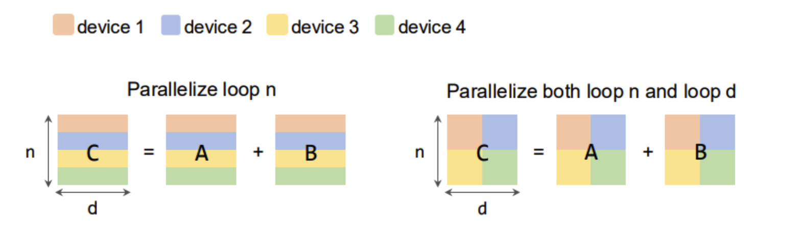
Matrix Multiplication
The outer loops (i, j) are independent and can be split across devices, but the reduction loop (k) introduces dependencies because partial results must be accumulated to compute C[i, j].
possible strategies:
-
split the rows of C and corresponding rows of A across devices, and replicate the full matrix B to each devices, so that each one could compute a subset of rows independently.
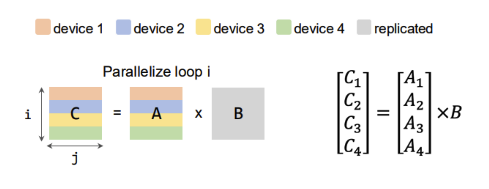
-
split matrix A among its columns, and split matrix B along its rows. Each device computes partial results for its assigned slice of A and B. After local computations, and all-reduce operation aggregates these partial results to produce the final matrix C.
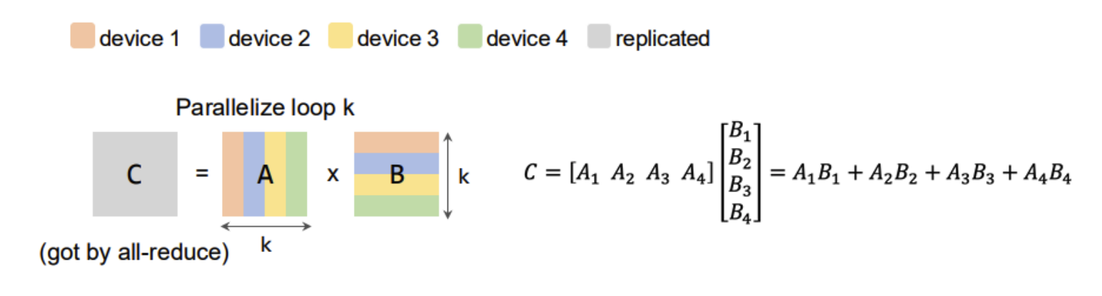
-
parallelize two loops together. The output matrix C is both column-partitioned and row-partitioned and is divided into 4 regions. Each device would compute a portion of C independently. The input matrices A and B are partially tiled to ensure all devices have the necessary data for their assigned computations. Similarly, we can parallelize both loop i and k, which results in a partially tiled matrix C. In this method we an all-reduce is needed to get matrix C.
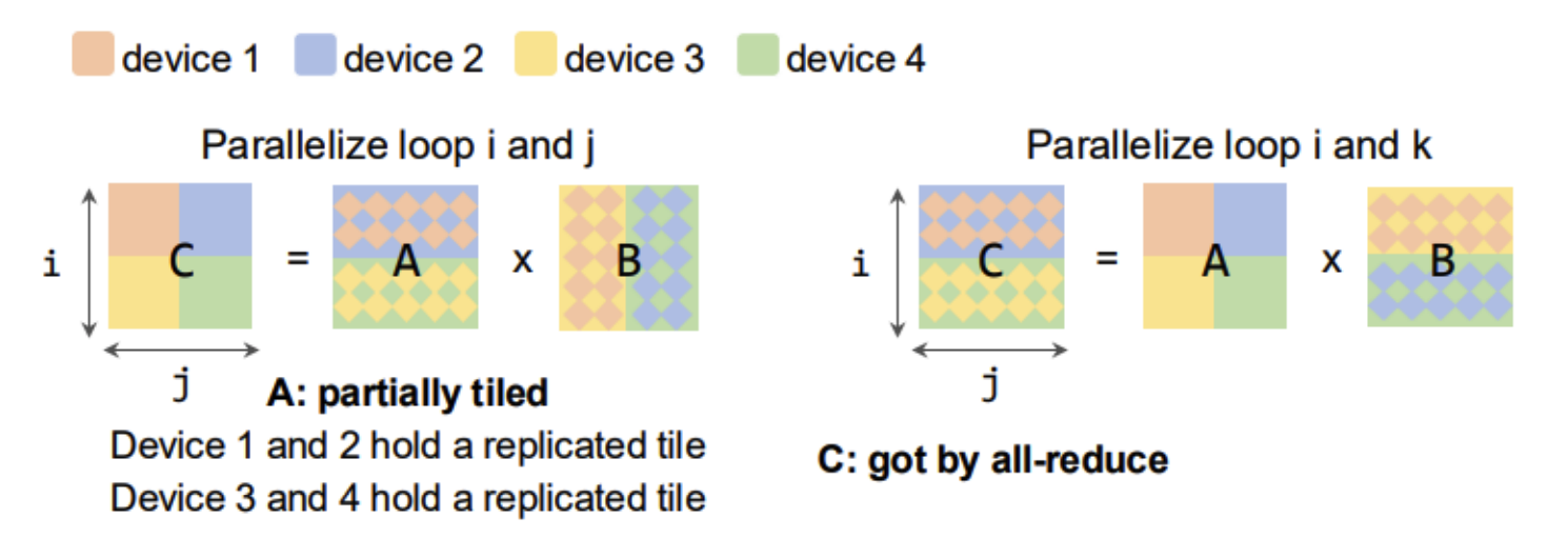
2D Convolution
In terms of 2D convolution operations, one simple way is to parallelize the batch dimension, output channels as well as input channels, and then the parallelization strategies are almost the same as matmul’s.
Two Intra-Op Parallelism strategies for matmul
Type 1: Partitioning Matmul Along Rows.
- In this case, no communication is needed.
- Input A is partitioned, and input B is replicated. The result matrix is composed of sub-regions.
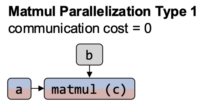
Type 2: Partitioning the Reduction Loop (K-Dimension).
- In this type, both inputs are partitioned along the reduction dimension.
- An all-reduce operation is required to complete the computation.
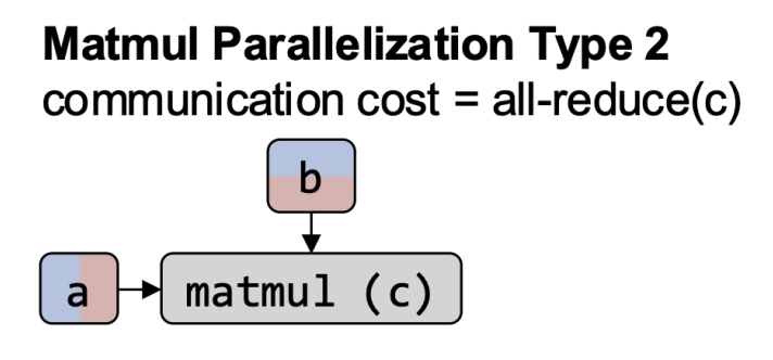
Computation Graph for a Two-Layer MLP
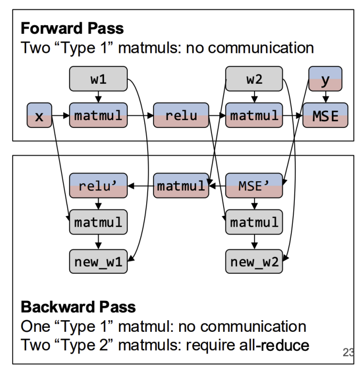
- Forward Pass
- Weight tensors W1 and W2 are replicated (data parallelism)
- Matmul and ReLU operations are partitioned along the batch dimension, requiring no communication.
- Backward Pass
- Contains one Type-1 matmul and two Type-2 matmuls.
- Some all-reduce operations on the gradients are required.
- Data parallelism necessitates communication due to specific partitioning choices.
Intra-Operator Parallelism, Repartitioning communication Cost and Optimization

- When applying intra-operator parallelism to an entire computational graph, there is a repartitioning communication cost on the edges.
- This arises because different operator parallelism strategies may require different partitioning formats for the same tensor, necessitating repartitioning.
To optimize the execution cost of the entire computational graph, it is crucial to strategically select partitioning strategies for each operator to minimize these repartitioning overheads when designing the partitioning scheme for the entire network.
When applying intra-operator parallelism to a whole graph, there is a repartitioning communication cost on the edges. Different operator parallelism strategies may require different tensor partitioning formats, necessitating repartitioning.
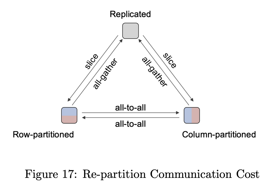
Optimization:
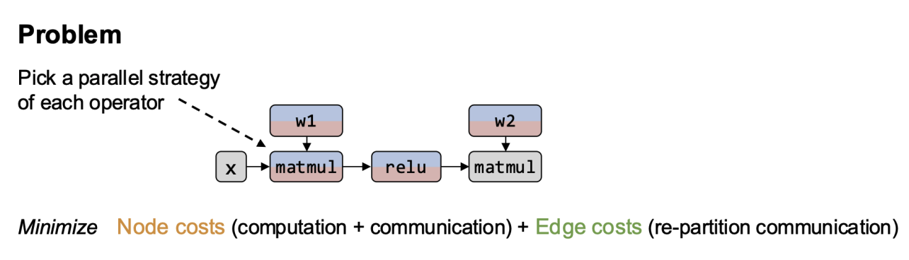
- Pick one parallel strategy per operator to minimize execution cost.
- Formulate the problem as an optimization:
- Select a coloring scheme for each node.
- Enumerate all possible communication costs.
- Minimize total cost to achieve efficient execution.
- possible approach:
- Manual design,
- Randomized search,
- Dynamic programming,
- Integer linear programming.
Intra-operator Parallelism Summary
- We can parallelize a single operator by exploiting its internal parallelism.
- To use intra-operator parallelism for a whole computational graph, we need to choose strategies for all nodes in the graph to minimize the communication cost.
- Intra-op and inter-op can be combined to achieve the best performance
In reality, we also want to combine the parallelization techniques with other techniques shown in previous lectures. We can do parallelization while also using other techniques, which includes:
- System-level Memory Optimizations: Rematerialization / Gradient Checkpointing, Swapping
- ML-level Optimizations: Quantization, Sparsification, Low-rank approximation
Few More Optimizations for parallelism
ZeRO Optimizer: Data Parallelism Optimization
The ZeRO (Zero Redundancy Optimizer) is an optimization technique designed to improve memory efficiency in large-scale distributed training.
- It addresses the inefficiencies of traditional data parallelism, which involves replicating optimizer states, gradients, and model weights across all devices, leading to excessive memory consumption.
Problem with Data Parallelism:
- In traditional data parallelism, all devices maintain a copy of: Optimizer states (which take significant memory, especially in large-scale models), Gradients, Model weights. This redundancy results in a large memory footprint and limits the scalability of deep learning models.
ZeRO Optimizer’s Idea
ZeRO optimizer aims to
- reduce memory usage by partitioning (instead of replicating) optimizer states, gradients, and model weights across devices.
- allows for more efficient utilization of memory and enables training larger models.
ZeRO Stages Overview
| Approach | Optimizer States (12M) | Gradients (2M) | Model Weights (2M) | Memory Cost | Communication Cost | |——————-|————————|—————-|———————|—————–|————————-| | Data Parallelism | Replicated | Replicated | Replicated | 16M | all-reduce(2M) | | ZeRO Stage 1 | Partitioned | Replicated | Replicated | 4M + 12M/N | all-reduce(2M) | | ZeRO Stage 2 | Partitioned | Partitioned | Replicated | 2M + 14M/N | all-reduce(2M) | | ZeRO Stage 3 | Partitioned | Partitioned | Partitioned | 16M/N | 1.5 all-reduce(2M) |
- Data Parallelism: High memory cost (16M) due to full replication.
- ZeRO Stage 1: Partitions optimizer states but keeps gradients and model weights replicated, reducing memory usage to 4M + 12M/N.
- ZeRO Stage 2: Further partitions gradients while keeping only model weights replicated, leading to 2M + 14M/N memory cost.
- ZeRO Stage 3: Fully partitions optimizer states, gradients, and model weights across devices, achieving the lowest memory cost (16M/N) and reducing communication cost.
ZeRO Stage 2 Overview
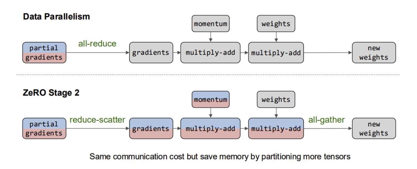
- Reduce-scatter: Distributes different portions of the gradients to different devices, avoiding full gradient replication.
- All-gather: Collects updated values from different devices after computation.
- This modification retains the same communication cost as all-reduce but significantly reduces memory consumption by partitioning more tensors.
Comparison between Data Parallelism and ZeRO Stage 2:
- Data Parallelism Workfow
- Partial Gradients Computation (on each device).
- All-reduce Operation: Each device receives the full set of gradients
- Momentum Update: The gradients are adjusted based on momentum.
- Weight Update: Weights are updated using gradients via multiply-add operations.
- New Weights Generation: The updated weights are used for the next iteration.
- ZeRO Stage 2 Workflow
- Partial Gradients Computation (on each device).
- Reduce-Scatter Operation: Gradients are partitioned across devices instead of being fully replicated.
- Momentum Update: Only the necessary portion of the gradients is updated per device.
- Weight Update: Each device computes weight updates on its partitioned gradients.
- All-Gather Operation: Updated gradients are assembled to produce new weights.
- Advantages of ZeRO Stage 2:
- Memory Efficiency: ZeRO Stage 2 significantly reduces memory usage by partitioning gradients alongside optimizer states.
- Scalability: Enables training larger models across multiple GPUs or nodes.
- Same Communication Cost: Despite gradient partitioning, the total communication cost remains unchanged compared to standard data parallelism.
ZeRO Stage 3 Overview
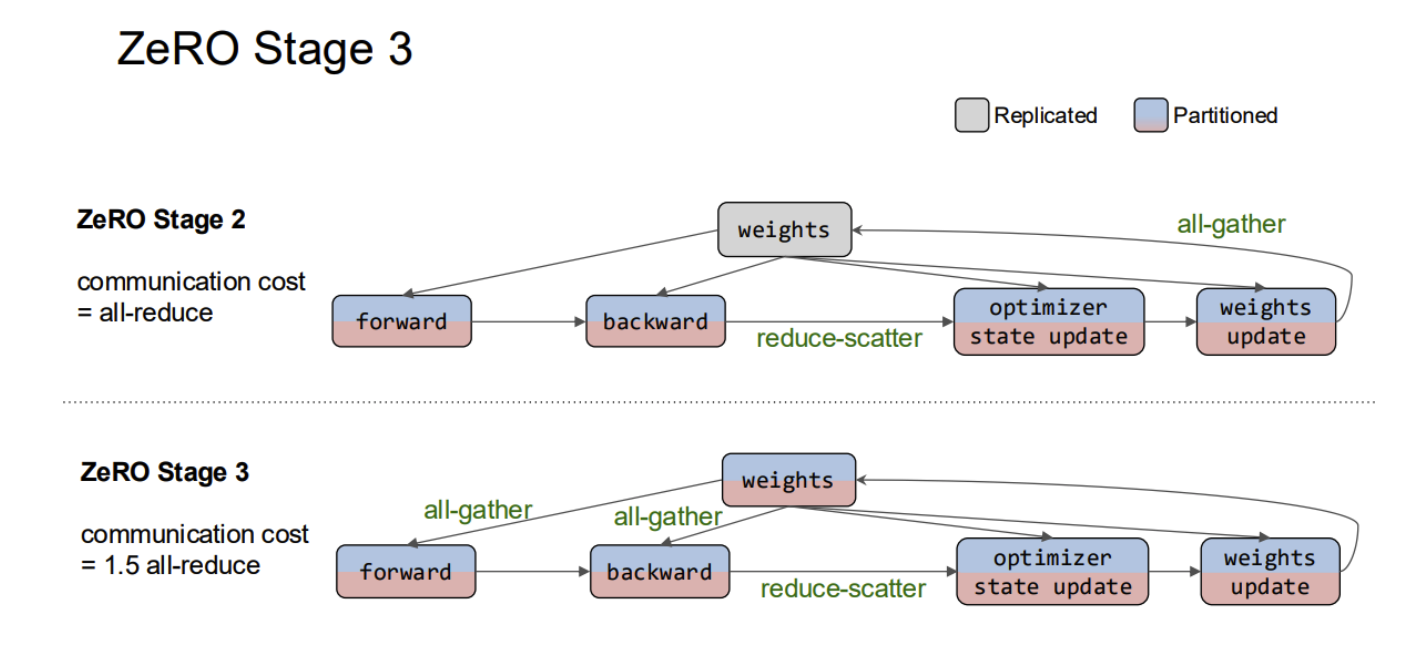
ZeRO Stage 3 builds upon ZeRO Stage 2 by fully partitioning optimizer states, gradients, and model weights, allowing deep learning models to scale further with minimal memory overhead.
The key difference in ZeRO Stage 3 is:
- ZeRO Stage 2: Uses all-reduce for communication.
- ZeRO Stage 3: Uses reduce-scatter and all-gather, leading to 1.5x all-reduce communication cost instead of 1x.
Comparison: ZeRO Stage 2 vs. ZeRO Stage 3
- ZeRO Stage 2 Workflow
- Forward Pass: Model processes input.
- Backward Pass: Computes gradients.
- Reduce-Scatter: Partitions and distributes gradient updates across devices.
- Optimizer State Update: Updates optimizer states (partitioned).
- Weights Update: Updates model weights (still replicated).
- All-Gather: Collects partitioned weights.
- ZeRO Stage 3 Workflow
- All-Gather Before Forward Pass: Since model weights are partitioned, an all-gather operation reconstructs weights before computation.
- Forward Pass: Model processes input.
- All-Gather Before Backward Pass: Partitioned weights are gathered again for gradient computation.
- Backward Pass: Computes gradients.
- Reduce-Scatter: Partitions gradient updates across devices.
- Optimizer State Update: Optimizer states are updated (partitioned).
- Weights Update: Partitioned weights are updated.
- Advantages of ZeRO Stage 3:
- Maximal Memory Efficiency: Fully partitions optimizer states, gradients, and model weights across devices.
- Enables Training of Billion-Scale Models: Makes it possible to train enormous models that wouldn’t fit into memory with traditional approaches.
- Trade-off Between Memory and Communication: While communication overhead increases (1.5x all-reduce), the memory footprint reduction allows training much larger models on fewer GPUs.
- Better GPU Utilization: Since memory usage is minimized, GPUs can handle larger batch sizes, improving throughput.
Mesh-TensorFlow: Mapping Tensor Dimensions to Mesh Dimensions
Tensor Dimensions
- Tensor dimensions are the axes along which data is organized in a tensor.
- Each tensor dimension represents a logical data axis in the computation.
- Using
mtf.Dimension(name, size)to define a tensor dimension.
Mesh Dimensions
- Mesh dimensions represent the distributed computational grid.
- They are defined using a list of tuples specifying the mesh dimension names and their sizes:
mesh_shape = [("rows", r), ("cols", c)]
Mapping Tensor Dimensions to Mesh Dimensions
Tensor dimensions are mapped to mesh dimensions using a computation layout. This mapping determines how tensors are distributed across the computation grid for efficient parallelism: computation_layout = [("batch", "rows"), ("hidden", "cols")]
This means:
- The “batch” dimension is distributed along “rows”.
- The “hidden” dimension is distributed along “cols”.
Summary:
- Mesh-TensorFlow enables explicit model parallelism by partitioning tensors across multiple devices.
- The tensor dimensions define the logical shape of data.
- The mesh dimensions represent the hardware topology.
- The mapping (computation layout) determines how tensor dimensions are split across available compute resources.
GSPMD
GSPMD is the successor of Mesh-TensorFlow.
- similar compiler-based approach.
- Users insert annotations to specify the parallelization strategy for important tensors.
- Later, the compiler propagates the strategy to the entire graph and generates SPMD (Single Program Multiple Data) parallel executables.
Combining Intra-op and Inter-op Parallelism
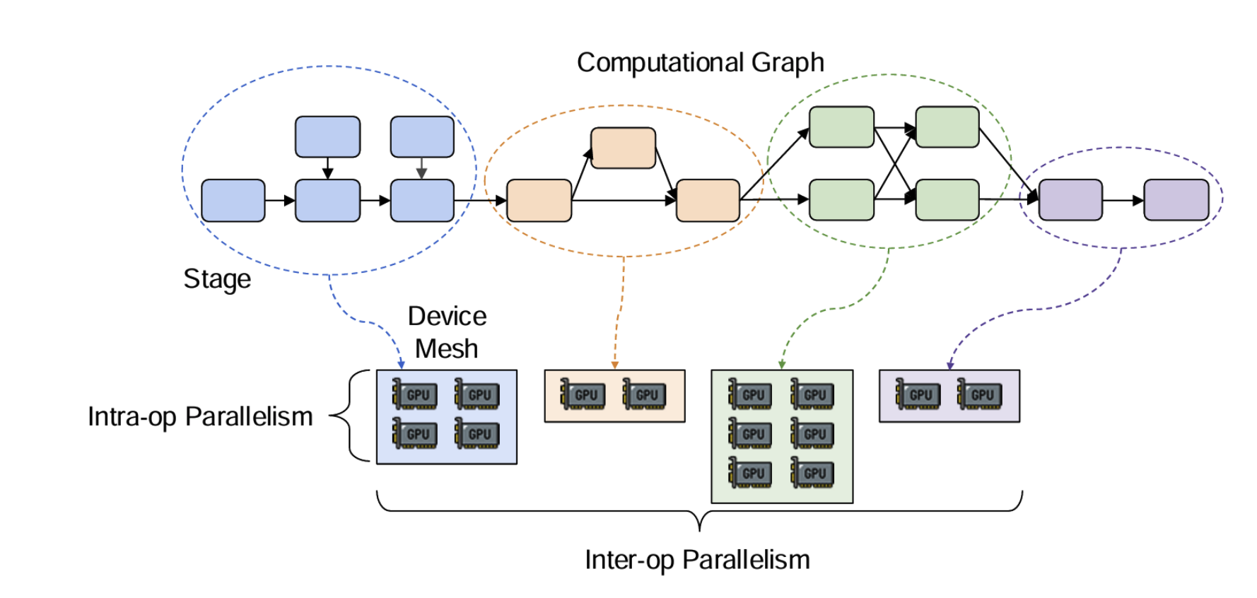
divide the computational graph into multiple stages and assign each stage to a different device mesh with different numbers of GPUs.
- keep the computational time approximately the same for each stage and benefits pipeline parallelism by reducing bubble size.
Auto-parallelization
Various parallelization techniques exist, including: Data Parallelism, Operator Partitioning, Pipeline Parallelism, ZeRO (Zero Redundancy Optimizer).
Different frameworks support these methods, such as:
- DeepSpeed, FairScale FSDP, Megatron-LM, Mesh-TF, GSPMD, GPipe, 1F1B
As models evolve from CNNs to large-scale architectures like BERT, GPT-3, and Mixture of Experts (MoE), the selection of an appropriate parallelization strategy becomes more complex. The key challenge for ML developers is: “Which parallelization strategy best fits my model and cluster?”
Problem Definition
max Performance(Model, Cluster), based on strategy ∈ Inter-op ∪ Intra-op
- Here, the goal is to maximize the training performance by selecting an optimal parallelization strategy from inter-operator (Inter-op) and intra-operator (Intra-op) parallelization methods.
Methods Overview
three categories of methods:
- Search-based methods: explore the parallelization space using techniques such as Markov Chain Monte Carlo (MCMC) and heuristics.
- Learning-based methods: These methods leverage machine learning techniques, including reinforcement learning, ML-based cost models, and Bayesian optimization, to guide the parallelization strategy.
- Optimization-based methods: These approaches formulate parallelization as an optimization problem and apply techniques such as dynamic programming, integer linear programming, and hierarchical optimization to find efficient solutions.
General Recipe for Automatic Parallelization
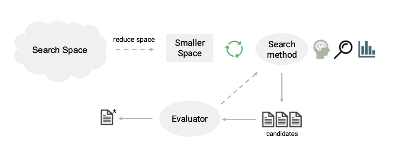
- Search Space: The initial set of all possible parallelization strategies.
- Space Reduction: Techniques are applied to prune infeasible or suboptimal strategies, reducing the search space.
- Search Method: A strategy is selected to explore the reduced space, which can involve heuristics, learning-based approaches, or optimization techniques.
- Evaluator: The performance of different strategies is assessed, and the best candidates are iteratively refined.
Examples
- Learning-based Method: ColocRL
- Optimization-based Method: Alpa
Hao’s ultimate guide
- Whether your model can fit into a single GPU?
- If yes, go to 2.
- If no, go to 3.
- Check the Job Completion Time (JCT) is acceptable.
- If JCT is acceptable, good to go.
- If not, data parallelism should be used until JCT is acceptable.
- check if memory optimization can make it fit: checkpoint rematerialization, gradient accumulation, and micro-batching. Usually swapping is avoided since it significantly slows down JCT.
- If yes, check JCT.
- If no or JCT is not acceptable, consider use intra-op and inter-op parallelism.
Once you have determined that parallelism is necessary, the next step is to assess GPU connectivity and bandwidth.
Parallelism to LLM training
Basic Concepts
Attention Mechanism
Input Layer with a Single Attention Layer
-
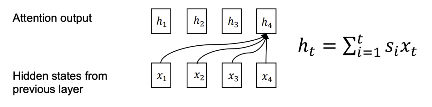
- Intuitively 𝑠𝑖 is “attention score” that computes how relevant the position 𝑖’s input is to this current hidden output Attention generally refers to weighted combination of individual states.
- usually stack multiple attention layers on top of this input, which are the hidden representations.
- Each state at the hidden token position attends to all previous layer states.
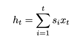
- The hidden states are calculated (as shown in the above formula) as the weighted sum of the product of the observation from the previous layer and the attention score si.
- This attention score, si, computes how relevant the position i’s input is to the current hidden output.
- There are different methods to decide how attention score is being computed, but the method we turn to is self-attention.
Self-Attention
At timestep t, with query qt, the self-attention output ht is computed in two steps:
- Compute pre-softmax attention scores:
- Compute weighted average of values using softmax-normalized scores:
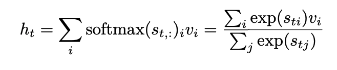
- Intuition: Attention scores sti quantify relevance of keys ki to the query qt. Then the values vi are aggregated proportionally to their computed relevance.
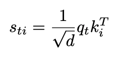
Multi-Head Attention
Multi-head attention introduces multiple attention heads (Q(j) , K(j) , V (j)) denotes the j-th attention head.
Each attention head operates independently, potentially capturing different types of relationships. Outputs from all heads are concatenated to form the final representation.
Transformer
Query, Key, and Value Vectors
𝑄 = 𝑋𝑊𝑞, 𝐾 = 𝑋𝑊𝑘, 𝑉 = 𝑋𝑊𝑣
Obtain 𝑄,𝐾,𝑉 from previous layer’s hidden state 𝑋 by linear projection
- 𝑊𝑞, 𝑊𝑘, 𝑊𝑣 are learned weight matrices
- X represents the input embeddings for the first layer, and for subsequent layers, X is the output from the previous layer.
- For multi-head attention, these projections are performed h times with different learned weight matrices, allowing the model to attend to different parts of the input space.
Transformer Block
𝑍 = SelfAttention(𝑋𝑊𝐾, 𝑋𝑊𝑄, 𝑋𝑊𝑉) 𝑍 = LayerNorm(𝑋 + 𝑍) 𝐻 = LayerNorm(ReLU(𝑍𝑊1)𝑊2 + 𝑍)
A typical transformer block comprises two main sublayers:
- a self-attention mechanism followed by
-
a positionwise feed-forward network, both wrapped with residual connections and layer normalization.
- The first equation computes the self-attention mechanism, transforming the input using the query, key, and value projections
- The second equation applies a residual connection (adding the original input X) followed by layer normalization, producing a normalized representation Z2
- The third equation represents a two-layer position-wise feed-forward network with ReLU activation, again followed by a residual connection and layer normalization
- The output H becomes the input for the next transformer block in the stack
Masked Self-Attention
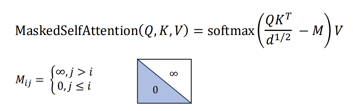
In language modeling tasks, we aim to model the conditional probability of each token given its preceding tokens.
This presents a fundamental challenge when training transformer models: while the entire sequence is available during training, the model must only access previous tokens when predicting the next token to avoid information leakage.
This constraint ensures the model learns to predict based solely on past context, as would be required during generation.
This effectively prevents each position from attending to future positions by setting their attention scores to −∞ before the softmax, resulting in attention weights of 0.
Feedforward Layer
A feedforward network (FFN) is composed of two linear transformations separated by a nonlinear activation function. Given an input x, we compute:
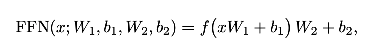
where W1 and W2 are weight matrices, b1 and b2 are bias vectors, and f is a nonlinear activation function (for instance, ReLU)
Transformer Summary
- Decoder-Centric: Decoder blocks are the fundamental components of language models, typically stacked in large numbers
- Core Components:
- Attention mechanisms (masked self-attention)
- Layer normalization
- Multi-layer perceptrons (MLPs)
- Input Processing:
- Token embeddings: Convert discrete tokens into continuous vector representations
- Positional embeddings: Encode sequential information (e.g., rotary embeddings)
- Training Objective: Cross-entropy loss with softmax applied over the sequence
Computing Components in LLM
- Element-wise operation
- layer normalization
- residual connection
- nonlinear activations,
- word embeddings,
- positional embeddings,
- loss function
- In contrast, MLPs and self-attention mechanisms can be more computationally intensive, because they involve matrix multiplications, which typically demand a large number of FLOPs
Connecting the Dots: Key Characteristic in Large Language Model
key characteristic when training large language models (LLMs):
- Compute: Estimating the number of floating-point operations (FLOPs) required for training.
- Memory: Ensuring that the memory usage does not exceed the GPU limits.
- Communication: Optimizing parallelization strategies
To analyze these three aspects, we need to consider the following
- Parameter Calculation for LLMs
- Memory: Allocating sufficient memory to store model parameters.
- Communication: When partitioning model weights, understanding their size helps determine an efficient partitioning strategy.
- FLOPs Estimation for Training
- Compute: Estimating the total computational cost required to complete the training process.
- Memory Estimation for Training
- Memory: Managing memory usage for storing parameters, intermediate activations, and optimizer states.
- Communication: If activation partitioning is employed, communication overhead should be considered.